
When a Data Studio (formerly Looker Studio) dashboard total differs from your Google Sheet after refreshing, check three mechanics: a chart, page, or report filter excluding rows; a percentage metric using SUM or AVG instead of a guarded SUM(discount_usd) / SUM(gross_sales_usd) calculated field; or order_id aggregated with COUNT_DISTINCT (orders) instead of COUNT (lines). Match filter scope across every metric and reconcile both dollars and counts.
Google reverted Looker Studio’s name to Data Studio in April 2026. Google Sheets is my preferred spreadsheet tool because a spreadsheet should be shareable whether you use it to collaborate or to communicate, and pairing Google Sheets with free Data Studio under an existing Google account lets you build these reports for $0 in extra software spend. I have seen numbers disagree across tools plenty of times. Once you know the data is fresh (see Why Your Data Studio Report Shows Old Data), the three steps below form the diagnostic path for this order-line example.
The Worked Order-Line Sheet (Order_Lines!A1:J8)
Here is a made-up April 2026 dataset with seven order lines across five distinct orders (ORD-701 to ORD-705) on a tab named Order_Lines (A1:J8). Row is a row-number guide; columns A:F are manual inputs, and columns G:J are formulas (the table shows their expected outputs; do not paste G2:J8 as constants):
| Row | line_id (A) | order_id (B) | order_date (C) | review_status (D) | gross_sales_usd (E) | discount_usd (F) | row_discount_rate (G) | net_sales_usd (H) | First_Order_Instance (I) | Cleared_First_Order_Instance (J) |
|---|---|---|---|---|---|---|---|---|---|---|
| 2 | LINE-01 | ORD-701 | 2026-04-05 | Cleared | $1,600.00 | $240.00 | 15.00% | $1,360.00 | 1 | 1 |
| 3 | LINE-02 | ORD-701 | 2026-04-05 | Cleared | $800.00 | $40.00 | 5.00% | $760.00 | 0 | 0 |
| 4 | LINE-03 | ORD-702 | 2026-04-12 | Cleared | $1,500.00 | $150.00 | 10.00% | $1,350.00 | 1 | 1 |
| 5 | LINE-04 | ORD-703 | 2026-04-19 | Cleared | $1,800.00 | $180.00 | 10.00% | $1,620.00 | 1 | 1 |
| 6 | LINE-05 | ORD-704 | 2026-04-30 | Pending_Review | $1,200.00 | $120.00 | 10.00% | $1,080.00 | 1 | 0 |
| 7 | LINE-06 | ORD-703 | 2026-04-19 | Cleared | $800.00 | $40.00 | 5.00% | $760.00 | 0 | 0 |
| 8 | LINE-07 | ORD-705 | 2026-04-30 | Cleared | $1,100.00 | $110.00 | 10.00% | $990.00 | 1 | 1 |
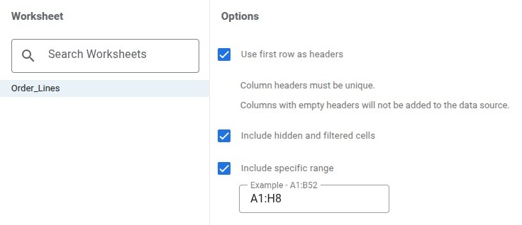
To keep inputs locale-safe in Google Sheets or Excel for the web, enter C2:C8 with =DATE(year,month,day) (=DATE(2026,4,5) to =DATE(2026,4,30), =COUNT(C2:C8) equals 7) and E2:F8 as plain numbers (1600, 240, etc., =COUNT(E2:E8) and =COUNT(F2:F8) equal 7) before formatting. In Data Studio’s Google Sheets connector (first-time setup: Build Your First Data Studio Report from Google Sheets), check Use first row as headers, check Include specific range (the docs’ Optional Range) set to A1:H8 (excluding I:J helpers and L1:Q10), and confirm field types (C:Date, A/B/D:Text, E/F/H:Currency, G:Percent). These formulas are a fixed 7-row demonstration; adding rows requires coordinated range and row-count (7) updates.
Across all 7 rows, gross sales total $8,800.00, discounts total $880.00 (10.00% weighted discount rate), and net sales total $7,920.00 across 5 orders. Row 6 (LINE-05, $1,080.00 net) is Pending_Review, while the other 6 rows are Cleared ($7,600.00 gross, $760.00 discount, $6,840.00 net across 4 Cleared orders). Enter these four formulas in G2:J2 and copy down through row 8:
- G2 (
row_discount_rate):
=IF(OR(TRIM(SUBSTITUTE(A2,CHAR(160)," "))="", TRIM(SUBSTITUTE(B2,CHAR(160)," "))="", C2="", NOT(ISNUMBER(C2)), TRIM(SUBSTITUTE(D2,CHAR(160)," "))="", NOT(EXACT(A2, UPPER(TRIM(SUBSTITUTE(A2, CHAR(160), " "))))), NOT(EXACT(B2, UPPER(TRIM(SUBSTITUTE(B2, CHAR(160), " "))))), NOT(EXACT(C2, TRIM(SUBSTITUTE(C2, CHAR(160), " ")))), NOT(EXACT(D2, TRIM(SUBSTITUTE(D2, CHAR(160), " ")))), ISNUMBER(SEARCH("~*", A2&B2&C2&D2)), ISNUMBER(SEARCH("~?", A2&B2&C2&D2)), ISNUMBER(SEARCH("~~", A2&B2&C2&D2)), LEN(A2)<>7, NOT(EXACT(LEFT(A2, 5), "LINE-")), NOT(ISNUMBER(SEARCH(MID(A2, 6, 1), "0123456789"))), NOT(ISNUMBER(SEARCH(MID(A2, 7, 1), "0123456789"))), LEN(B2)<>7, NOT(EXACT(LEFT(B2, 4), "ORD-")), NOT(ISNUMBER(SEARCH(MID(B2, 5, 1), "0123456789"))), NOT(ISNUMBER(SEARCH(MID(B2, 6, 1), "0123456789"))), NOT(ISNUMBER(SEARCH(MID(B2, 7, 1), "0123456789"))), AND(NOT(EXACT(D2, "Cleared")), NOT(EXACT(D2, "Pending_Review"))), NOT(ISNUMBER(E2)), NOT(ISNUMBER(F2)), SUMPRODUCT(--EXACT($A$2:$A$8, A2))>1), "CHECK INPUTS", IF(OR(C2<DATE(2000,1,1), INT(C2)<>C2, E2<0, F2<0, F2>E2), "CHECK INPUTS", IF(E2=0, 0, ROUND(F2/E2, 4))))
- H2 (
net_sales_usd):
=IF(NOT(ISNUMBER(G2)), "CHECK INPUTS", ROUND(E2 - F2, 2))
- I2 (
First_Order_Instance):
=IF(OR(NOT(ISNUMBER(H2)), COUNT($H$2:$H$8)<7), "CHECK INPUTS", IF(SUMPRODUCT(--EXACT($B$2:B2, B2))=1, 1, 0))
- J2 (
Cleared_First_Order_Instance):
=IF(OR(NOT(ISNUMBER(H2)), COUNT($H$2:$H$8)<7), "CHECK INPUTS", IF(AND(EXACT(D2, "Cleared"), SUMPRODUCT(--EXACT($B$2:B2, B2), --EXACT($D$2:D2, "Cleared"))=1), 1, 0))
Per Google’s COUNTIF and EXACT documentation, ordinary <> comparisons are case-insensitive (without wildcard matching), whereas COUNTIF is case-insensitive and interprets * and ? as wildcards and ~ as an escape character. If you test mistyping B8 (ORD-705) as ORD-70? on a copy, COUNTIF($B$2:B8, B8) matches all 7 ORD-70x rows and drops distinct orders from 5 to 4. In G2, the OR(...) guard combines EXACT, explicit */?/~ checks (SEARCH("~*", ...)), and SEARCH digit checks so any non-canonical or wildcard-containing ID returns "CHECK INPUTS" before I2:J8 accept the table. Restore B8 to ORD-705 after testing.

Step 1: Align Filter Scope Across Every Metric (Col M vs. Col N)
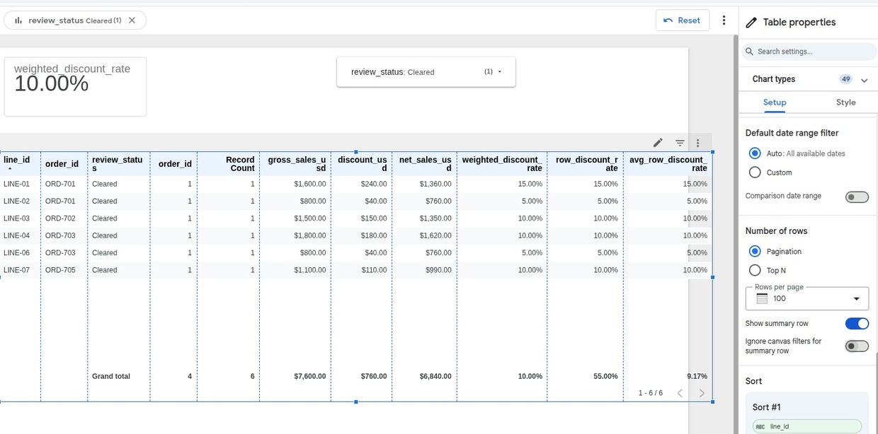
When your Data Studio scorecard shows $6,840.00 net sales while =SUM(H2:H8) shows $7,920.00, inspect active filter properties: check the Applied filters panel, the chart’s Filter section, Page > Current page settings > Setup, File > Report settings, Resource > Manage filters, and Default date range (verifying whether filter inheritance is enabled on each chart).
Here, Include review_status = "Cleared" excludes Row 6 (LINE-05, $1,080.00 net). Never delete a legitimate business filter just to match an unfiltered =SUM(H2:H8):
- Accidental leftover filter: Remove it and compare every scorecard against
Col M(All_Rows_Sheet_Benchmark: $8,800.00 gross, $880.00 discount, $7,920.00 net, 10.00% rate, 7 lines, 5 orders). - Intentional business filter: Keep it on the dashboard and compare every metric against
Col N(Cleared_Sheet_Benchmark: $7,600.00 gross, $760.00 discount, $6,840.00 net, 10.00% rate, 6 lines, 4 orders).
Also check worksheet filters: =SUM(H2:H8) includes rows hidden by Data > Create a filter, whereas =SUBTOTAL(109, H2:H8) sums only visible rows. In the Google Sheets connector, Include hidden and filtered cells applies to manually hidden rows and ordinary sheet filters, whereas Google Sheets Filter views never filter Data Studio.
Step 2: Replace AVG or SUM of Percentages With a Guarded SUM/SUM Field
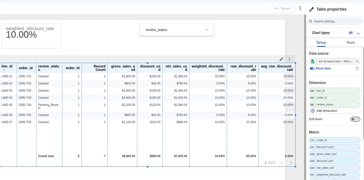
Always inspect and explicitly set each metric’s aggregation (Sum, Average, Count Distinct, or Count) in the chart or data source rather than assuming a default. When row_discount_rate (Col G) is aggregated as Sum, a scorecard shows 65.00% across all 7 rows; switched to Average (AVG), it shows 9.29% across all 7 rows (or 9.17% across the 6 Cleared rows). As Why You Should Not Average Margin Percentages explains, averaging row percentages weights an $800.00 line the same as an $1,800.00 line; see Percentage Change vs Percentage Points when describing rate gaps.
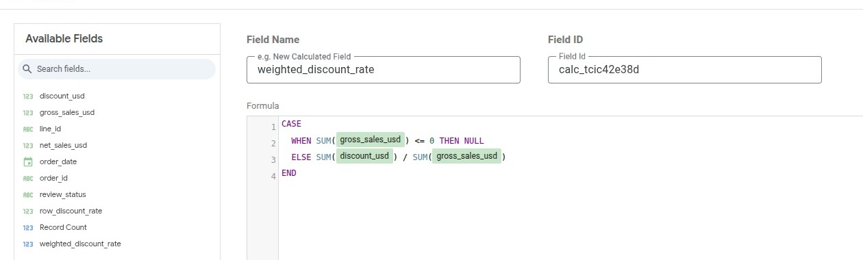
Per Data Studio’s calculated fields documentation, create a data-source calculated field (Resource > Manage added data sources > Edit > Add a field) with a zero-denominator guard:
CASE
  WHEN SUM(gross_sales_usd) <= 0 THEN NULL
  ELSE SUM(discount_usd) / SUM(gross_sales_usd)
END
This Auto-aggregated field computes the revenue-weighted discount rate for the active scope (10.00% across all 7 rows $880 / $8,800; 10.00% across the 6 baseline Cleared rows $760 / $7,600; 8.67% across the 5 Cleared rows $520 / $6,000 if LINE-01 is also Pending_Review; 15.00% on LINE-01 alone; 11.67% on ORD-701).
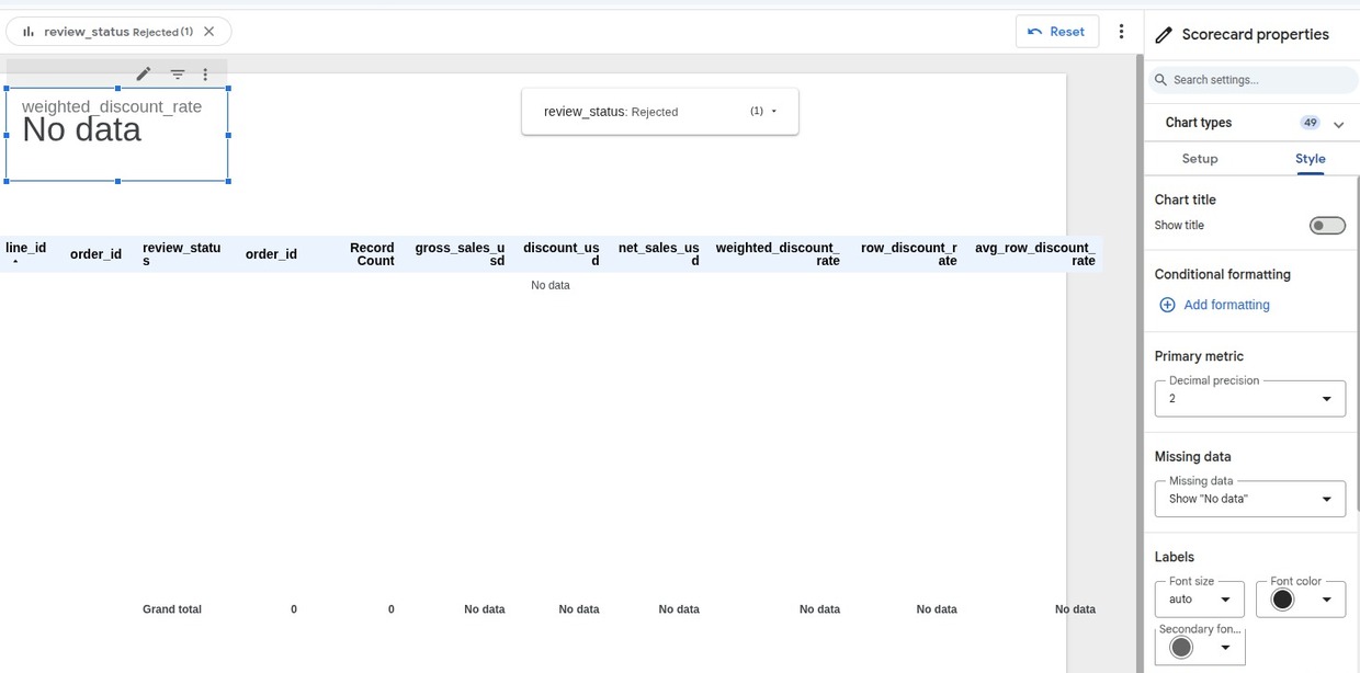
When a filter matches 0 rows or gross sales are zero, 0/0 is undefined and the CASE expression evaluates to NULL. Per Data Studio’s Scorecard reference, missing-data rendering is configurable under Style > Missing Data—set it to Show “No data” rather than “0” so NULL is never mistaken for a valid 0% rate. In the sheet, an empty Cleared subset (D2:D8 all set to Pending_Review) turns N2:N10 and any observed column referencing $N$ into "CHECK INPUTS", while M2:M10 and any column referencing $M$ remain valid ($7,920.00 net, 10.00% rate, 7 lines, 5 orders).
Step 3: Match Identifier Grain (COUNT_DISTINCT vs. COUNT) With Scope-Aware Counters
In Order_Lines, each row is an order line, not an order header; see What Does One Row Represent in Your Sales Spreadsheet? and Duplicate Sales Rows or Legitimate Order Lines?. Inspect your scorecard metric explicitly: set order_id to Count Distinct (CTD) to count orders (5 across 7 lines, or 4 across 6 Cleared lines), and use Record Count or line_id set to Count to count lines (7 or 6).
In the spreadsheet, never count distinct orders in a filtered subset by summing the unfiltered First_Order_Instance flag (Col I) inside SUMIFS. Test why on a copy: set D2 (LINE-01, first line of ORD-701) to Pending_Review while leaving D3 (LINE-02, second line of ORD-701) as Cleared. Because I2=1 is on the Pending_Review row and I3=0 is on the Cleared row, SUMIFS(I2:I8, D2:D8, "Cleared") returns 3 instead of 4. Column J (Cleared_First_Order_Instance) flags the first Cleared line of each order (J2=0, J3=1), so =SUM($J$2:$J$8) still returns 4 ($6,000.00 gross, $520.00 discount, $5,480.00 net, 8.67% rate, 5 Cleared lines). Restore D2 to Cleared when finished.
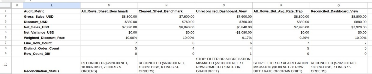
Build the Dual-Benchmark Reconciliation Block (Order_Lines!L1:Q10)
Leave column K blank and place this 9-row block in L1:Q10. Columns M and N are live benchmarks (M10 and N10 confirm benchmark validity, not dashboard verification). Columns O, P, and Q operate in Observed-Input Mode, showing three expected synthetic scenarios (O = leftover Cleared filter + AVG rate; P = filter removed for all 7 rows, but AVG rate still used; Q = reconciled all-row dashboard). In your own audit, replace the six manual input rows (Rows 2, 3, 4, 6, 7, 8) with values independently read from Data Studio charts at the same date and filter scope (enter Row 6 rates as decimals like 0.0917 or percentages like 9.17%, never 10; leave unknown metrics blank or "TBD", never copied from M or N):
| Row | Audit_Metric (L) | All_Rows_Sheet_Benchmark (M) | Cleared_Sheet_Benchmark (N) | Unreconciled_Dashboard_View (O) | All_Rows_But_Avg_Rate_Trap (P) | Reconciled_Dashboard_View (Q) |
|---|---|---|---|---|---|---|
| 2 | Gross_Sales_USD | $8,800.00 | $7,600.00 | $7,600.00 | $8,800.00 | $8,800.00 |
| 3 | Discount_USD | $880.00 | $760.00 | $760.00 | $880.00 | $880.00 |
| 4 | Net_Sales_USD | $7,920.00 | $6,840.00 | $6,840.00 | $7,920.00 | $7,920.00 |
| 5 | Net_Variance_USD | $0.00 | $0.00 | -$1,080.00 | $0.00 | $0.00 |
| 6 | Weighted_Discount_Rate | 10.00% | 10.00% | 9.17% | 9.29% | 10.00% |
| 7 | Line_Row_Count | 7 | 6 | 6 | 7 | 7 |
| 8 | Distinct_Order_Count | 5 | 4 | 4 | 5 | 5 |
| 9 | Row_Count_Diff | 0 | 0 | 1 | 0 | 0 |
| 10 | Reconciliation_Status | RECONCILED ($7920.00 NET, 10.00% DISC, 7 LINES / 5 ORDERS) | RECONCILED ($6840.00 NET, 10.00% DISC, 6 LINES / 4 ORDERS) | STOP: FILTER OR AGGREGATION MISMATCH (-$1080.00 NET / 1 ROWS OMITTED / RATE OR GRAIN DRIFT) | STOP: FILTER OR AGGREGATION MISMATCH ($0.00 NET / 0 ROW DIFF / RATE OR GRAIN DRIFT) | RECONCILED ($7920.00 NET, 10.00% DISC, 7 LINES / 5 ORDERS) |
| Reconciliation Rule / Probe | Benchmark & Formula Behavior |
|---|---|
Invalid source data or zero all-row gross (A2:J8) |
M2:M10, N2:N10, and formula rows 5, 9, 10 in O:Q all return "CHECK INPUTS". |
Comparing an observed column against Col N (Cleared_Sheet_Benchmark) |
Replace $M$2, $M$3, $M$4, $M$6, $M$7, and $M$8 with $N$2, $N$3, $N$4, $N$6, $N$7, and $N$8 across all three formula rows (Rows 5, 9, and 10) in that column; manual cells (Rows 2, 3, 4, 6, 7, 8) remain manual inputs. |
Signed net variance & row-count direction (O10:Q10) |
Row 9 (Row_Count_Diff) computes $M$7 - O7 (>0 = ROWS OMITTED, <0 = EXTRA ROWS, 0 = 0 ROW DIFF), and Row 10 prints -$, +$, or $ so positive and negative gaps never flip sign. For example, setting E2 from 1600 to 2000 while Col Q stays at $7,920.00 net makes Q10 report STOP: FILTER OR AGGREGATION MISMATCH (-$400.00 NET / 0 ROW DIFF / RATE OR GRAIN DRIFT) (restore E2 to 1600 afterward). Aggregate reconciliation confirms summary totals, rates, and counts—not row-by-row identity or source completeness. |
Frequently Asked Questions
Why does a Data Studio table’s Summary row not equal the sum or average of the rows above it?
Per Data Studio’s Table reference, a table’s Summary row evaluates each metric’s formula across the active dataset rather than summing displayed rows vertically. Keep Ignore canvas filters in summary row unchecked so the summary row inherits the same report, page, and control filters as the table (producing 10.00% across all 7 rows or across the 6 baseline Cleared rows, even though ORD-701 is 11.67% and LINE-01 is 15.00%).
What to Do Next
For broader timing and system boundary issues, read Why Your Business Numbers Don’t Match Across Systems. When combining tables before building a dashboard, check Append vs Merge: How Should You Combine Tables? and Why Merging Tables Inflates Your Sales Total, cross-check totals with Build a Monthly Sales Pivot Table in Google Sheets, and publish metrics in How to Build a Monthly KPI Scorecard.
Copy-Paste Formula Reference
M2:M10 (All_Rows_Sheet_Benchmark) and N2:N10 (Cleared_Sheet_Benchmark):
- M2:
=IF(OR(COUNTA($A$2:$A$8)<7, COUNT($C$2:$C$8)<>COUNTA($A$2:$A$8), COUNT($E$2:$E$8)<>COUNTA($A$2:$A$8), COUNT($F$2:$F$8)<>COUNTA($A$2:$A$8), COUNT($G$2:$G$8)<7, COUNT($H$2:$H$8)<7, COUNT($I$2:$I$8)<7, COUNT($J$2:$J$8)<7, COUNTIF($G$2:$G$8, "CHECK INPUTS")>0, COUNTIF($H$2:$H$8, "CHECK INPUTS")>0, COUNTIF($I$2:$I$8, "CHECK INPUTS")>0, COUNTIF($J$2:$J$8, "CHECK INPUTS")>0, SUM($E$2:$E$8)<=0), "CHECK INPUTS", ROUND(SUM($E$2:$E$8), 2))
- M3:
=IF(NOT(ISNUMBER($M$2)), "CHECK INPUTS", ROUND(SUM($F$2:$F$8), 2))
- M4:
=IF(NOT(ISNUMBER($M$2)), "CHECK INPUTS", ROUND(SUM($H$2:$H$8), 2))
- M5:
=IF(NOT(ISNUMBER($M$2)), "CHECK INPUTS", 0)
- M6:
=IF(OR(NOT(ISNUMBER($M$2)), NOT(ISNUMBER($M$3))), "CHECK INPUTS", IF($M$2<=0, "CHECK INPUTS", ROUND($M$3 / $M$2, 4)))
- M7:
=IF(NOT(ISNUMBER($M$2)), "CHECK INPUTS", COUNTA($A$2:$A$8))
- M8:
=IF(NOT(ISNUMBER($M$2)), "CHECK INPUTS", SUM($I$2:$I$8))
- M9:
=IF(NOT(ISNUMBER($M$2)), "CHECK INPUTS", 0)
- M10:
=IF(OR(NOT(ISNUMBER($M$2)), NOT(ISNUMBER(M5)), NOT(ISNUMBER(M6)), NOT(ISNUMBER(M7)), NOT(ISNUMBER(M8)), NOT(ISNUMBER(M9))), "CHECK INPUTS", "RECONCILED ($" & TEXT(M4, "0.00") & " NET, " & TEXT(M6, "0.00%") & " DISC, " & M7 & " LINES / " & M8 & " ORDERS)")
- N2:
=IF(OR(COUNTA($A$2:$A$8)<7, COUNT($C$2:$C$8)<>COUNTA($A$2:$A$8), COUNT($E$2:$E$8)<>COUNTA($A$2:$A$8), COUNT($F$2:$F$8)<>COUNTA($A$2:$A$8), COUNT($G$2:$G$8)<7, COUNT($H$2:$H$8)<7, COUNT($I$2:$I$8)<7, COUNT($J$2:$J$8)<7, COUNTIF($G$2:$G$8, "CHECK INPUTS")>0, COUNTIF($H$2:$H$8, "CHECK INPUTS")>0, COUNTIF($I$2:$I$8, "CHECK INPUTS")>0, COUNTIF($J$2:$J$8, "CHECK INPUTS")>0, SUMPRODUCT(--EXACT($D$2:$D$8, "Cleared"))=0), "CHECK INPUTS", IF(SUMIFS($E$2:$E$8, $D$2:$D$8, "Cleared")<=0, "CHECK INPUTS", ROUND(SUMIFS($E$2:$E$8, $D$2:$D$8, "Cleared"), 2)))
- N3:
=IF(NOT(ISNUMBER($N$2)), "CHECK INPUTS", ROUND(SUMIFS($F$2:$F$8, $D$2:$D$8, "Cleared"), 2))
- N4:
=IF(NOT(ISNUMBER($N$2)), "CHECK INPUTS", ROUND(SUMIFS($H$2:$H$8, $D$2:$D$8, "Cleared"), 2))
- N5:
=IF(NOT(ISNUMBER($N$2)), "CHECK INPUTS", 0)
- N6:
=IF(OR(NOT(ISNUMBER($N$2)), NOT(ISNUMBER($N$3))), "CHECK INPUTS", IF($N$2<=0, "CHECK INPUTS", ROUND($N$3 / $N$2, 4)))
- N7:
=IF(NOT(ISNUMBER($N$2)), "CHECK INPUTS", SUMPRODUCT(--EXACT($D$2:$D$8, "Cleared")))
- N8:
=IF(NOT(ISNUMBER($N$2)), "CHECK INPUTS", SUM($J$2:$J$8))
- N9:
=IF(NOT(ISNUMBER($N$2)), "CHECK INPUTS", 0)
- N10:
=IF(OR(NOT(ISNUMBER($N$2)), NOT(ISNUMBER(N5)), NOT(ISNUMBER(N6)), NOT(ISNUMBER(N7)), NOT(ISNUMBER(N8)), NOT(ISNUMBER(N9))), "CHECK INPUTS", "RECONCILED ($" & TEXT(N4, "0.00") & " NET, " & TEXT(N6, "0.00%") & " DISC, " & N7 & " LINES / " & N8 & " ORDERS)")
O5, O9, O10 (copy across O:Q; replace $M$2, $M$3, $M$4, $M$6, $M$7, $M$8 with $N$2, $N$3, $N$4, $N$6, $N$7, $N$8 across all three rows for Col N):
- O5 (
Net_Variance_USD):
=IF(OR(NOT(ISNUMBER($M$2)), NOT(ISNUMBER(O2)), NOT(ISNUMBER(O3)), NOT(ISNUMBER(O4)), NOT(ISNUMBER($M$4))), "CHECK INPUTS", IF(OR(O2<=0, O3<0, O3>O2, ROUND(O2-O3, 2)<>ROUND(O4, 2)), "CHECK INPUTS", ROUND(O4 - $M$4, 2)))
- O9 (
Row_Count_Diff):
=IF(OR(NOT(ISNUMBER($M$2)), NOT(ISNUMBER(O7)), NOT(ISNUMBER($M$7)), NOT(ISNUMBER(O8))), "CHECK INPUTS", IF(OR(O7<=0, INT(O7)<>O7, O8<=0, INT(O8)<>O8, O8>O7), "CHECK INPUTS", $M$7 - O7))
- O10 (
Reconciliation_Status):
=IF(OR(NOT(ISNUMBER($M$2)), NOT(ISNUMBER(O5)), NOT(ISNUMBER(O6)), NOT(ISNUMBER($M$6)), NOT(ISNUMBER(O7)), NOT(ISNUMBER(O8)), NOT(ISNUMBER(O9))), "CHECK INPUTS", IF(OR(O6<0, O6>1), "CHECK INPUTS", IF(OR(ROUND(ABS(O2-$M$2), 2)>0, ROUND(ABS(O3-$M$3), 2)>0, ROUND(ABS(O5), 2)>0, O9<>0, ROUND(ABS(O6-$M$6), 4)>0, O7<>$M$7, O8<>$M$8), "STOP: FILTER OR AGGREGATION MISMATCH (" & IF(ROUND(O5, 2)<0, "-$", IF(ROUND(O5, 2)>0, "+$", "$")) & TEXT(ABS(O5), "0.00") & " NET / " & IF(O9>0, O9 & " ROWS OMITTED", IF(O9<0, ABS(O9) & " EXTRA ROWS", "0 ROW DIFF")) & " / RATE OR GRAIN DRIFT)", "RECONCILED ($" & TEXT(O4, "0.00") & " NET, " & TEXT(O6, "0.00%") & " DISC, " & O7 & " LINES / " & O8 & " ORDERS)")))