Build Your First Data Studio Report from Google Sheets

Connect a Google Sheet to Data Studio, build two Scorecards, a monthly Time Series and a category Table, then check every chart against totals calculated in the sheet to catch total rows and out-of-window dates.

To build your first Data Studio report from Google Sheets, keep your data as a flat table with one header row and no total rows inside the range. Select Create > Report, choose the Google Sheets connector, pick your tab, and check Use first row as headers. Add two Scorecards, a monthly Time Series, and a category Table. Then check each chart against totals you calculate in the sheet.

Data Studio was called Looker Studio from October 2022 until April 2026, so you will see both names in menus and search results (Welcome to Data Studio). I prefer Google Sheets because a spreadsheet should be shareable, whether you use it to collaborate or to communicate. Connecting it to Data Studio needs no additional BI subscription for this example.

The Two Report Mistakes This Example Catches

Here is a made-up invoice log on a tab named Sales_Source: seven January–February 2026 invoices totaling $10,500.00. Columns A to E are the raw data you connect. Columns F and G are audit helpers from Step 1, kept outside the connected range. The Row column is a row-number guide, not a worksheet column.

Enter B2:B8 as real dates, such as =DATE(2026,1,6) in B2, formatted yyyy-mm-dd. Enter the seven amounts in E2:E8 as plain numbers (2200, not "$2,200"), formatted as currency. Formatting does not turn pasted text into numbers, so confirm =COUNT(B2:B8) and =COUNT(E2:E8) both return 7.

Row	invoice_id (A)	invoice_date (B)	customer_name (C)	service_category (D)	net_sales_usd (E)	Report_Month (F)	Row_Source_Audit (G)
2	INV-5901	2026-01-06	Apex Property Group	Installation	$2,200.00	2026-01	VALID SOURCE ROW
3	INV-5902	2026-01-14	Beacon Retail LLC	Maintenance	$1,400.00	2026-01	VALID SOURCE ROW
4	INV-5903	2026-01-24	Cedar Ridge Medical	Repair	$1,200.00	2026-01	VALID SOURCE ROW
5	INV-5904	2026-02-04	Harbor View Hotel	Installation	$1,800.00	2026-02	VALID SOURCE ROW
6	INV-5905	2026-02-12	Summit Logistics Co	Maintenance	$1,700.00	2026-02	VALID SOURCE ROW
7	INV-5906	2026-02-19	Northstar Dental	Repair	$1,000.00	2026-02	VALID SOURCE ROW
8	INV-5907	2026-02-26	Oakwood Industrial	Installation	$1,200.00	2026-02	VALID SOURCE ROW

The F and G values are what the Step 1 formulas should return, not values to type. Test each mistake on a copy, or reset as shown in Step 3:

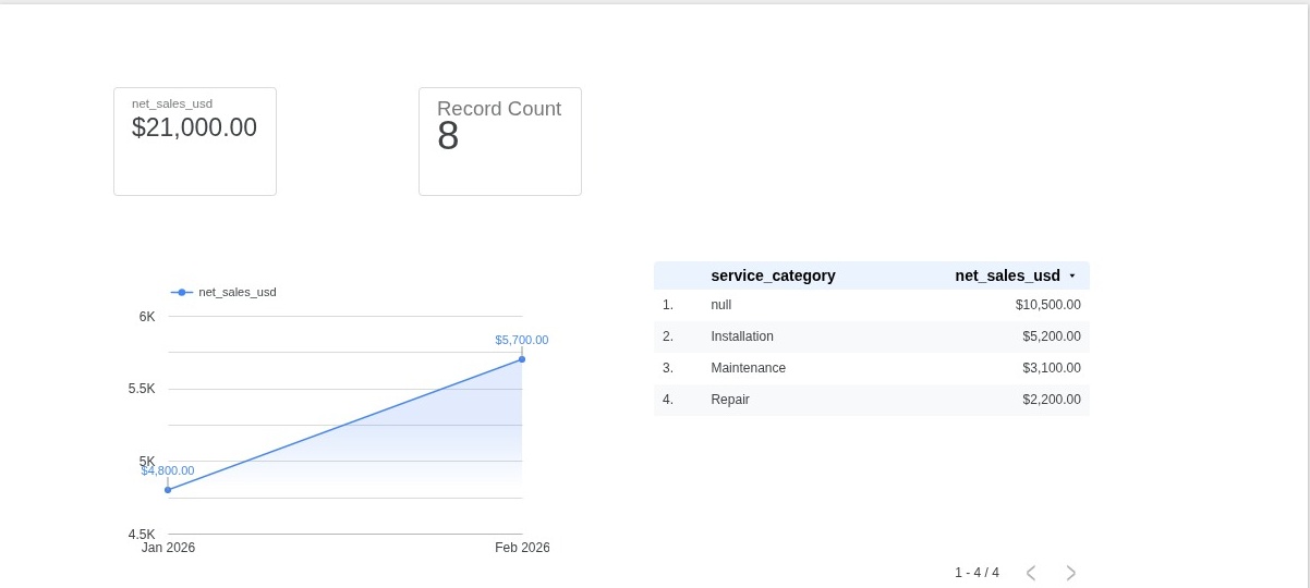
A total row inside the range. Add TOTAL in A9 and 10500 in E9, then connect A1:E9. Data Studio reads every row as a record (Google’s Sheets data-source tutorial), so Net Sales doubles to $21,000.00 and Record Count reads 8. The Jan–Feb Time Series and the three named categories still add up to $10,500.00, because the total row has no date or category.
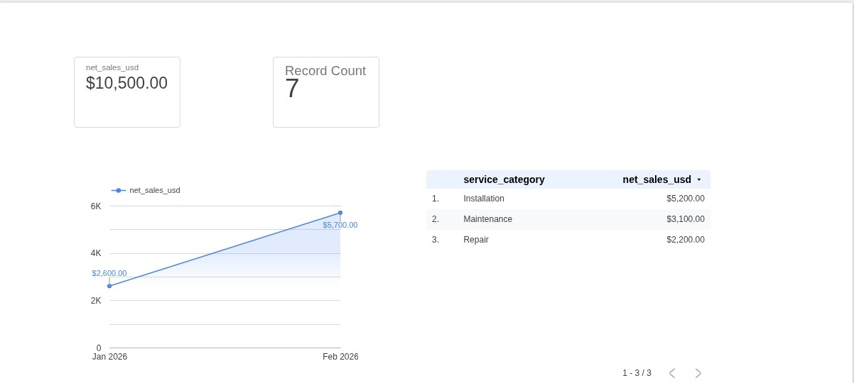
A date outside the report window. Change B2 to =DATE(2026,3,6). The Scorecards still read $10,500.00 and 7, and the categories still add up to $10,500.00. The Jan–Feb Time Series drops to $2,600.00 and $5,700.00, or $8,300.00. The $2,200.00 March invoice is missing.

With a TOTAL row inside the connected range, net sales double to $21,000.00 and Record Count reads 8, while the monthly points stay at $4,800.00 and $5,700.00. Open full-size image.

With one invoice dated in March, the Scorecards and categories still show $10,500.00, but the January–February Time Series adds up to only $8,300.00. Open full-size image.

Step 1: Prepare the Sheet and Add Audit Helpers

Check four things on Sales_Source before you connect:

One header row. Field names sit in A1:E1, with no merged title rows above them.
One invoice per row. Every row in A2:E8 is one customer invoice (what one row represents in your sales spreadsheet), with no total or subtotal rows.
Helpers stay outside the connection. Data Studio can import formula columns, but this example connects only the raw data in A1:E8. Keep F1:G8 and the check block in I1:K12 outside that range.
Two helper columns. Enter these formulas in F2 and G2, then fill them down to row 8:

=IF(OR(TRIM(A2)="", UPPER(TRIM(A2))="TOTAL", TRIM(C2)="", TRIM(D2)="", NOT(ISNUMBER(B2)), NOT(ISNUMBER(E2))), "CHECK INPUTS", IF(OR(B2<DATE(2000,1,1), E2<0), "CHECK INPUTS", TEXT(B2, "yyyy-mm")))

=IF(UPPER(TRIM(A2))="TOTAL", "SUMMARY ROW IN RANGE (REMOVE)", IF(F2="CHECK INPUTS", "CHECK INPUTS", IF(COUNTIF($A$2:$A$8, A2)>1, "DUPLICATE INVOICE ID", IF(NOT(OR(D2="Installation", D2="Maintenance", D2="Repair")), "INVALID CATEGORY", IF(NOT(OR(F2="2026-01", F2="2026-02")), "OUT OF REPORT WINDOW", "VALID SOURCE ROW")))))

F2 returns the invoice month, or "CHECK INPUTS" when a field is blank, the row says TOTAL, or the date or amount is not a number. It tests for numbers before it checks ranges. G2 gives total rows, input errors, duplicate IDs and unknown categories their own labels, separate from "OUT OF REPORT WINDOW".

Step 2: Connect the Sheet and Build Four Visuals

Follow Google’s Sheets connector guide:

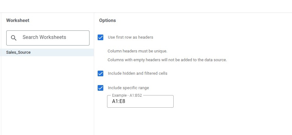
Select Create > Report, choose the Google Sheets connector, and pick your workbook and the Sales_Source tab. Check Use first row as headers, leave Include hidden and filtered cells checked, check Include specific range, enter A1:E8, and click Add.
Confirm invoice_date is Date, net_sales_usd is Currency (USD) with Sum aggregation (Aggregation reference), and the other fields are Text.

Four visuals keep the page focused (how many KPIs a small business should track). Add each with Add a chart, then use the Setup and Style tabs:

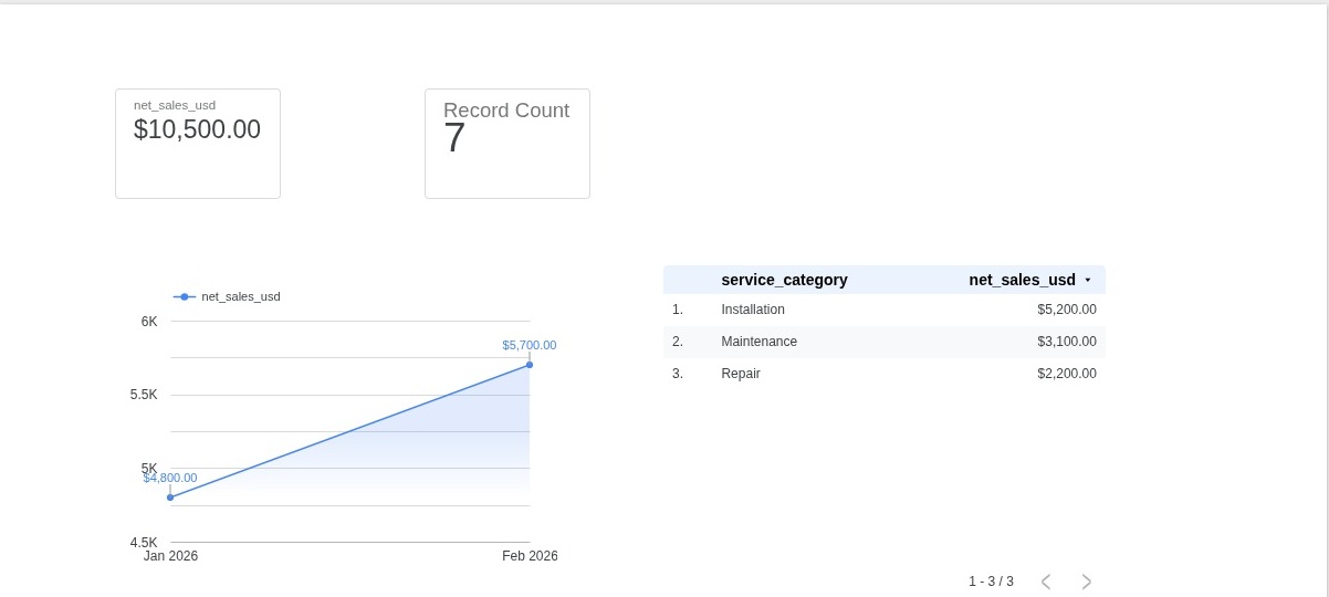
Net Sales Scorecard (Scorecard reference). Choose Scorecard and set Metric to net_sales_usd. Leave Default date range on Auto, which covers the sheet’s full date span (report date ranges), and add no filters. In Style, uncheck Compact numbers and set Decimal precision to 2, so you read $10,500.00, not 10.5K.
Record Count Scorecard. Add a second Scorecard the same way, with Metric Record Count and Decimal precision 0.
Monthly Time Series (Time Series reference). Choose Time series. Set Date range dimension and Dimension to invoice_date at Year Month granularity, and set Metric to net_sales_usd. Set its Default date range to Custom, Jan 1 to Feb 28, 2026. Skip page-wide date controls, which would filter the Scorecards too. In Style, check Show data labels, uncheck Compact numbers, and set Decimal precision to 2. Read the point labels, not the rounded axis.
Category Table (Table reference). Choose Table, set Dimension to service_category and Metric to net_sales_usd, and leave the date range on Auto so March stays in. In Style, uncheck Compact numbers. Read only the three named rows, ignoring any summary row or blank/null row a total row creates.

The Google Sheets connector set to Sales_Source, first row as headers, and the specific range A1:E8. Open full-size image.

The four visuals on the clean sheet: $10,500.00 across seven invoices, with the monthly points and category rows adding up to the same total. Open full-size image.

Step 3: Check the Report Against the Sheet

Build this check block in Sales_Source!I1:K12. Column J calculates what each chart should show. Column K holds what you read off the report, and rows 9 to 12 compare them. The K values shown are expected readings for this made-up example; enter your actual readings.

Row	Check (I)	Sheet_Benchmark (J)	Report_Reading (K)
2	Scorecard_Net_Sales_USD	$10,500.00	$10,500.00
3	Scorecard_Record_Count	7	7
4	Time_Series_Jan_2026_USD	$4,800.00	$4,800.00
5	Time_Series_Feb_2026_USD	$5,700.00	$5,700.00
6	Category_Installation_USD	$5,200.00	$5,200.00
7	Category_Maintenance_USD	$3,100.00	$3,100.00
8	Category_Repair_USD	$2,200.00	$2,200.00
9	Breakdown_Gap_USD		$0.00
10	Total_Variance_USD		$0.00
11	Record_Count_Diff		0
12	Status		RECONCILED: 4 VISUALS MATCH SHEET ($10,500.00)

The made-up invoice log with its audit helpers and the I1:K12 check block after entering the clean report readings. Open full-size image.

Each label before = names the destination cell; paste only the formula. First, the benchmarks:

J2: =IF(OR(COUNTA($A$2:$A$8)<7, COUNT($B$2:$B$8)<7, COUNT($E$2:$E$8)<7, COUNTIF($F$2:$F$8, "CHECK INPUTS")>0, COUNTIF($G$2:$G$8, "VALID SOURCE ROW")+COUNTIF($G$2:$G$8, "OUT OF REPORT WINDOW")<7), "CHECK INPUTS", ROUND(SUM($E$2:$E$8), 2))
J3: =IF(NOT(ISNUMBER(J2)), "CHECK INPUTS", COUNTA($A$2:$A$8))
J4: =IF(NOT(ISNUMBER($J$2)), "CHECK INPUTS", ROUND(SUMIFS($E$2:$E$8, $F$2:$F$8, "2026-01"), 2))
J6: =IF(NOT(ISNUMBER($J$2)), "CHECK INPUTS", ROUND(SUMIFS($E$2:$E$8, $D$2:$D$8, "Installation"), 2))

Copy J4 into J5 and change "2026-01" to "2026-02". Copy J6 into J7 and J8, and change the category to "Maintenance" and "Repair".

Then the four checks:

K9: =IF(OR(NOT(ISNUMBER(J2)), COUNT(K2:K8)<7), "CHECK INPUTS", IF(OR(K3<0, K3<>INT(K3)), "CHECK INPUTS", ROUND(MAX(ABS(K2 - (K4 + K5)), ABS(K2 - (K6 + K7 + K8))), 2)))
K10: =IF(OR(NOT(ISNUMBER(K9)), NOT(ISNUMBER(J2))), "CHECK INPUTS", ROUND(K2 - J2, 2))
K11: =IF(NOT(ISNUMBER(K9)), "CHECK INPUTS", ABS(K3 - COUNTIF($G$2:$G$8, "VALID SOURCE ROW")))
K12: =IF(NOT(ISNUMBER(K11)), "CHECK INPUTS", IF(K10<>0, "STOP: $" & TEXT(ABS(K10), "#,##0.00") & IF(K10>0, " INFLATED (", " TOTAL VARIANCE (") & IF(J2=0, "ZERO BENCHMARK", IF(K10>0, "+", "") & TEXT(K10/J2, "0.00%")) & " / " & K11 & " RECORD COUNT DIFF)", IF(K9<>0, "STOP: $" & TEXT(K9, "#,##0.00") & " BREAKDOWN GAP (" & K11 & " RECORD COUNT DIFF)", IF(OR(K11<>0, K3<>J3), "STOP: $0.00 VARIANCE (" & K11 & " RECORD COUNT DIFF)", IF(OR(ROUND(K4-J4,2)<>0, ROUND(K5-J5,2)<>0, ROUND(K6-J6,2)<>0, ROUND(K7-J7,2)<>0, ROUND(K8-J8,2)<>0), "STOP: CHART MISMATCH VS SHEET", "RECONCILED: 4 VISUALS MATCH SHEET ($" & TEXT(K2, "#,##0.00") & ")")))))

Leave K2:K8 blank until you read the report; the checks show "CHECK INPUTS" until all seven readings are numbers. K9 counts numeric readings before testing for a whole-number record count, so text such as "TBD" never reaches INT.

K9, breakdown gap: the larger difference between the Scorecard total and the monthly points or category rows.
K10, total variance: report total minus sheet total.
K11, record-count difference: the absolute difference between Record Count and the rows column G marks "VALID SOURCE ROW". It compares report and sheet; it does not identify a faulty row. A reading of 8 on a clean seven-row sheet gives 1.
K12, status: RECONCILED only when all three checks are zero and every reading matches its benchmark.

Run the two tests, then reset

Columns J and K recalculate from the live sheet, so reread the report after each change:

Total-row test: Add TOTAL in A9 and 10500 in E9. Open the data source, click Edit connection, change Include specific range to A1:E9, click Reconnect, then Apply (edit the data source connection). Refresh and enter the readings. K12 should read STOP: $10,500.00 INFLATED (+100.00% / 1 RECORD COUNT DIFF). Then clear A9:E9 and set the range back to A1:E8 the same way.
March test: Change B2 to =DATE(2026,3,6), refresh, and enter the new readings. G2 shows "OUT OF REPORT WINDOW", leaving six valid rows, so K12 reads STOP: $2,200.00 BREAKDOWN GAP (1 RECORD COUNT DIFF). Then change B2 back to =DATE(2026,1,6).
Clean check: With both changes undone, refresh, re-enter all seven readings, and confirm K12 reads RECONCILED: 4 VISUALS MATCH SHEET ($10,500.00).

Limits of This Check

This example is fixed to A1:E8 and January–February 2026. Refresh data and Refresh fields do not grow the range. To reuse the sheet, extend each range that ends at row 8: the connector, the F:G fill, the duplicate check in G2, and the ranges in J2:J8 and K11. Change the four 7s in the J2 guard to your row count, update the months in G2, J4 and J5 and the Time Series range, then check again.

A clean result shows that totals, months, categories and record count match the sheet. It does not prove each row matches, since two invoices can share an amount, month and category, or that every billed invoice is in the sheet.

Troubleshooting

Symptom	Cause	Fix
Scorecard reads $21,000.00 and Record Count reads 8	A `TOTAL` row sits inside the connected range	Delete the total row and set the connector range back to `A1:E8`
Scorecard reads $10,500.00, but Jan + Feb add up to $8,300.00	An invoice date falls outside Jan–Feb 2026	Look for `"OUT OF REPORT WINDOW"` in column G and correct the date
Edited sheet values do not appear in Data Studio yet	Sheets data is cached for 15 minutes by default (Manage data freshness)	Click More options > Refresh data to request fresh data
New or renamed headers in row 1 do not appear	Refresh data updates values, not field names	Open the data source and click Refresh fields

Frequently Asked Questions

How often does a Google Sheets report in Data Studio update its numbers?

Sheets connections use a 15-minute cache by default (Manage data freshness). An uncached query fetches sooner, and Refresh data requests fresh data on demand.

Does matching Record Count and Count Distinct prove my report is complete?

No. If Record Count and Count Distinct (CTD) of invoice_id both read 7, the connected IDs are unique. That does not prove every billed invoice is in the sheet or that each row is one invoice. Tie the total to your billing system for the same period.

What to Do Next

To summarize monthly totals in the sheet first, build a monthly sales pivot table in Google Sheets. Once your visuals reconcile, organize your metrics with a monthly KPI scorecard and check your layout against 7 dashboard mistakes small businesses make.