
To build your first Power BI sales report from Excel, format your order rows as a named Excel Table with no total row inside it. In Power BI Desktop, select Home > Excel workbook, check the table (not the sheet) in Navigator, and click Load. Build five visuals: a Net Sales Card, two order-count Cards, a monthly column chart, and a channel Table. Then check every reading against Excel.
My preferred tool is Google Sheets because a spreadsheet should be shareable. It should be easy to collaborate and communicate with others. The Google version of this tutorial is Build Your First Data Studio Report from Google Sheets. If your business runs on Microsoft 365, start with what you already have: Excel plus Power BI Desktop, a free Windows download. I’d keep data-tool spend at $0 for as long as the office suite you already run can do the job (how much a small business should spend on data tools). Paid licenses come in when you share reports through the Power BI service, which Is Power BI Worth It for a Small Business? covers.
The Power BI readings and check results below come from a test of this exact workbook in Excel and Power BI Desktop (version 2.152, March 2026 release) on Windows in US English. The one exception is the wording of the success message, explained in Step 4. Menus move between releases, so expect small label differences.
The Example and the Mistakes It Catches
Below is the Excel table I made up for this article. It holds seven January–February 2026 orders on a sheet named Sales_Source, totaling $12,400.00. Columns A to E are the order data. Columns F and G are audit helpers, and they stay outside the table. The Row column is a row-number guide, not a worksheet column.
| Row | order_id (A) | order_date (B) | customer_name (C) | sales_channel (D) | net_sales_usd (E) | Report_Month (F) | Row_Source_Audit (G) |
|---|---|---|---|---|---|---|---|
| 2 | ORD-6901 | 2026-01-08 | Alder Industrial Supply | Direct | $2,100.00 | 2026-01 | VALID SOURCE ROW |
| 3 | ORD-6902 | 2026-01-16 | Bramble Logistics Group | Partner | $1,900.00 | 2026-01 | VALID SOURCE ROW |
| 4 | ORD-6903 | 2026-01-27 | Crestview Clinics LLC | Renewal | $1,400.00 | 2026-01 | VALID SOURCE ROW |
| 5 | ORD-6904 | 2026-02-05 | Dunbar Equipment Co | Direct | $2,400.00 | 2026-02 | VALID SOURCE ROW |
| 6 | ORD-6905 | 2026-02-13 | Elmwood Dental Partners | Partner | $2,000.00 | 2026-02 | VALID SOURCE ROW |
| 7 | ORD-6906 | 2026-02-20 | Fairview Cold Storage | Renewal | $1,000.00 | 2026-02 | VALID SOURCE ROW |
| 8 | ORD-6907 | 2026-02-26 | Granite Ridge Builders | Direct | $1,600.00 | 2026-02 | VALID SOURCE ROW |
January comes to $5,400.00 and February to $7,000.00. By channel, Direct is $6,100.00, Partner $3,900.00, and Renewal $2,400.00. The report should show exactly these numbers.
The test caught three kinds of mistakes:
- Extra rows in the load. A total row inside the table, whether you type it or turn on Excel’s built-in Total Row, doubles Net Sales to $24,800.00. Loading the whole sheet instead of the table pulls in helper columns and blank rows.
- Two years in one January. If one order is dated January 2025, a month-only chart merges it with January 2026, and the bar still looks right.
- A rounded Card. The default Card showed 12K, not $12,400.00. Copy that number into a check, and you are $400.00 off.
Step 1: Format the Orders as a Named Excel Table
Put the headings in A1:E1 and the seven orders in rows 2 to 8. Enter dates as real dates and amounts as plain numbers (2100, not “$2,100”). Then confirm =COUNT(B2:B8) and =COUNT(E2:E8) both return 7. If a count is short, some cells hold text that only looks like a date or number (fix date locale before building a monthly report).
Next, turn the range into a table (Overview of Excel tables):
- Click any cell in
A1:E8and select Home > Format as Table (or press Ctrl+T). Check My table has headers. - On the Table Design tab, set Table Name to
Sales_Orders.
Now add the two helper columns. Paste the F2 and G2 formulas from the formula reference at the end of this article, then fill both down to row 8. F2 returns the order month, or "CHECK INPUTS" when a field is blank or the wrong type, the ID is not in the ORD-0000 pattern, the row says TOTAL, or the amount has fractions of a cent. G2 labels each row: a total row, a duplicate ID, an unknown channel, and a date outside January–February 2026 each get their own label. All seven rows should read "VALID SOURCE ROW".
Excel can grow a table when you type or paste right next to it (resize a table). In the test, typing a single 0 in E9 pulled row 9 into Sales_Orders and moved the formula ranges with it. So check the table’s edges after the helpers are in, right before you save:
- Select Table Design > Resize Table and confirm the range reads
$A$1:$E$8. If the table stretched over columns F and G, set it back here. - Leave Total Row unchecked on the Table Design tab. In the test, Power BI loaded Excel’s built-in total row as an eighth order, and Net Sales read $24,800.00.
- Save the workbook.
Do any experiment on a copy of the workbook, never on the file your report reads.
Step 2: Load Only the Table in Power BI Desktop
Microsoft’s Excel report tutorial covers the same connection steps:
- Open Power BI Desktop, select Home > Excel workbook, and pick your file.
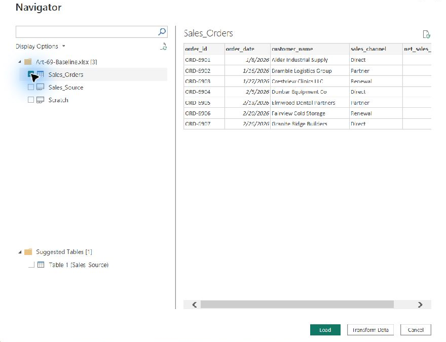
- Navigator lists
Sales_Orderswith a table icon andSales_Sourcewith a sheet icon. It may also offer a Suggested Tables entry. Check onlySales_Orders, then click Load. - Open Table view from the left rail. The status bar at the bottom should read
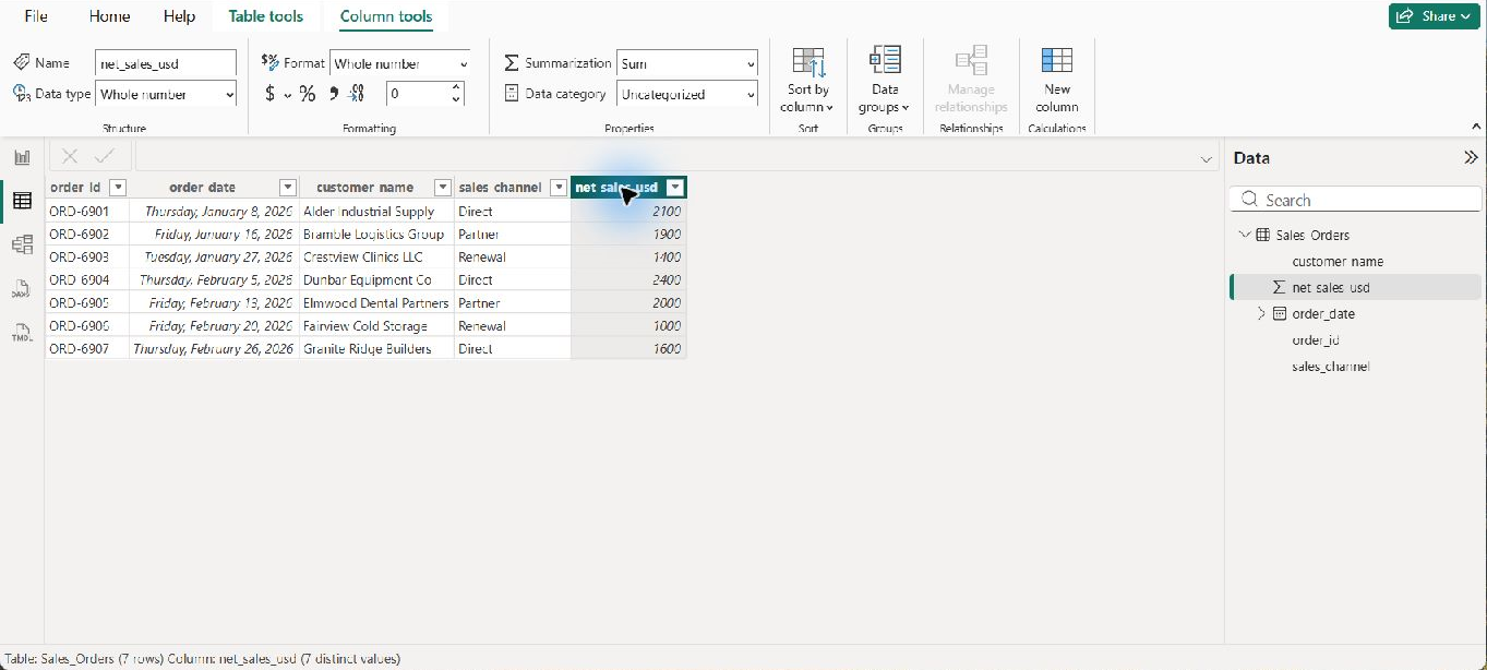
Table: Sales_Orders (7 rows), and the table should have five columns,order_idthroughnet_sales_usd. Step 4 explains why the row count matters even when every total matches.
Picking the sheet is the easy mistake. In the test, loading Sales_Source as a sheet gave 11 columns and 12 rows after Power BI promoted the headers (Excel connector). It contained the seven orders, the helper and check columns, and five rows with no order ID from the check block. Power BI also guessed that the Report_Month helper text was a date. Net Sales still read $12,400.00, so the total alone would not have warned you.
Then check types and formatting:
- In the Data pane,
order_dateshould show a calendar icon andnet_sales_usda sum (∑) icon. - Power BI typed
net_sales_usdas Whole number in the test because every amount is whole dollars. That is fine for this example. If your own amounts have cents, click Transform Data before loading and check the type Power Query assigns, so the cents survive the import (Power Query data types). Currency formatting changes only how the number looks. - With
net_sales_usdselected, set Column tools > Format to Currency,$ English (United States), with 2 decimal places. - If
order_datehas no date hierarchy under it, open File > Options and settings > Options > Current File > Data Load and check Auto date/time in the Time intelligence section (Auto date/time in Power BI Desktop). Microsoft says it is on by default in a new installation, but a global setting can turn it off for new files.
Step 3: Build Five Visuals
Click the empty canvas before adding each visual so Power BI doesn’t replace the selected visual with the new one.
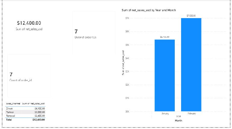
- Net Sales Card. Add a Card and check
net_sales_usd, which Power BI sums. In the test, the Card first showed 12K. Under Format visual > Callout value, set Display units to None. That was the path in the tested Card; newer Card versions may show Callout values > Values instead (card visual guide). The Card then read $12,400.00. The stored total never changed; only the display did. - Order Count Card. Add a second Card and drag
order_idinto its field well. Open the field’s drop-down and choose Count. It reads 7. - Distinct ID Card. Add a third Card with
order_idand choose Count (Distinct) (aggregates in Power BI). It also reads 7. Rename the field for this visual, for example “Distinct order IDs”, so you can tell the two Cards apart. - Monthly column chart. Add a Clustered column chart. Put
order_dateon the X-axis and remove Quarter and Day from its hierarchy, so Year and Month remain. Putnet_sales_usdon the Y-axis. Turn on Data labels and set their display units to None. - Channel Table. Add a Table with
sales_channelandnet_sales_usd. Its rows read $6,100.00, $3,900.00, and $2,400.00, with a $12,400.00 total.
The two count Cards answer different questions. Count skips blank IDs. Count (Distinct) counts each different value once, and Microsoft’s DISTINCTCOUNT reference says a blank counts as one more value. So a duplicate order ID pushes Count above Count (Distinct), and a row with no ID pushes Count (Distinct) above Count. The tested report keeps the two counts on separate Cards. For why one row should mean one order, see what one row represents in your sales spreadsheet.
The chart needs one more decision. It opens at the Year level, and Microsoft’s drill mode guide describes two ways down to months. Expanding all down one level in the hierarchy keeps Year and Month together: January 2026 reads $5,400.00 and February 2026 reads $7,000.00. Going to the next level in the hierarchy drops the year, so January 2025 and January 2026 would share one bar. Use Expand all down, and hover over the icons on the chart’s header to find it.
Before you read any numbers, click the empty canvas to clear any cross-filter. Then confirm the Filters pane shows no active filters.
Step 4: Check Every Reading Against Excel
Build this check block in Sales_Source!I1:K13. Column J calculates what each visual should show. Column K holds what you read off the report. Rows 10 to 13 compare them. The K values shown are the clean readings from the test; enter your own.
| Row | Check (I) | Excel_Benchmark (J) | Report_Reading (K) |
|---|---|---|---|
| 2 | Card_Net_Sales_USD | $12,400.00 | $12,400.00 |
| 3 | Card_Nonblank_Order_IDs | 7 | 7 |
| 4 | Card_Distinct_Order_IDs | 7 | 7 |
| 5 | Chart_Jan_2026_USD | $5,400.00 | $5,400.00 |
| 6 | Chart_Feb_2026_USD | $7,000.00 | $7,000.00 |
| 7 | Table_Direct_USD | $6,100.00 | $6,100.00 |
| 8 | Table_Partner_USD | $3,900.00 | $3,900.00 |
| 9 | Table_Renewal_USD | $2,400.00 | $2,400.00 |
| 10 | Breakdown_Gap_USD | $0.00 | |
| 11 | Total_Variance_USD | $0.00 | |
| 12 | Nonblank_ID_Count_Diff | 0 | |
| 13 | Reconciliation_Status | RECONCILED: REPORT MATCHES EXCEL ($12,400.00) |
Paste J2:J9 and K10:K13 from the formula reference, one cell at a time. Leave K2:K9 blank until you read the report. Until all eight readings are numbers, rows 10 to 13 show "CHECK INPUTS". Type each reading as a plain number: 12400, not “12K” and not text. In the test, a 7 typed with a leading apostrophe was stored as text, and the checks stopped with "CHECK INPUTS".
K10, breakdown gap: the larger difference between the Net Sales Card and either the two month bars or the three channel rows.K11, total variance: report total minus Excel total.K12, count difference: how far the Count Card is from the Excel ID count and from the rows column G marks"VALID SOURCE ROW".K13, status: saysRECONCILEDonly when all three checks are zero, the two counts agree, and every reading matches its benchmark. Otherwise it names the first problem it finds.
I renamed the success message for this article. The tested workbook printed RECONCILED: 4 VISUALS MATCH EXCEL ($12,400.00); the formula below prints RECONCILED: REPORT MATCHES EXCEL ($12,400.00), so the message does not depend on how many visuals you build. The checks themselves are unchanged.
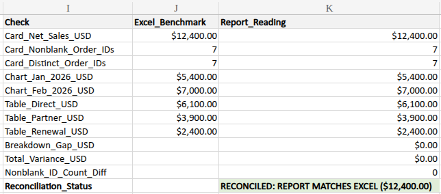
Here is what the checks showed when each mistake was loaded into Power BI. Counts are Count, then Count (Distinct). Rows are the number in the Table view status bar. The clean row shows the renamed success message.
For the source-data cases, the setup was the same. Power BI read a fresh copy holding only columns A to E, with the table resized to include any extra rows. The readings went into the check block of a separate, clean workbook. In your regular workbook, extra rows would trip the J2 guard and every check would show "CHECK INPUTS" instead. The two date rows are the exception: there, B2 changed in both files. Start each case from a fresh copy.
| What changed | Net Sales | Counts | Rows | K13 result |
|---|---|---|---|---|
| Nothing (clean table) | $12,400.00 | 7 / 7 | 7 | RECONCILED: REPORT MATCHES EXCEL ($12,400.00) |
Typed TOTAL row with 12400 loaded as row 9 |
$24,800.00 | 8 / 8 | 8 | STOP: $12,400.00 INFLATED (+100.00% / 1 NONBLANK ID COUNT DIFF) |
| Same total row with the ID cell left blank | $24,800.00 | 7 / 8 | 8 | STOP: $12,400.00 INFLATED (+100.00% / 0 NONBLANK ID COUNT DIFF) |
Extra $0 order ORD-6908 |
$12,400.00 | 8 / 8 | 8 | STOP: $0.00 VARIANCE (1 NONBLANK ID COUNT DIFF) |
| Extra $0 row with no ID | $12,400.00 | 7 / 8 | 8 | STOP: BLANK ORDER ID IN REPORT (7 NONBLANK VS 8 DISTINCT) |
ORD-6907 loaded twice |
$14,000.00 | 8 / 7 | 8 | STOP: DUPLICATE ORDER IDS IN REPORT (8 NONBLANK VS 7 DISTINCT) |
A $0 copy of ORD-6907 plus a $0 row with no ID |
$12,400.00 | 8 / 8 | 9 | STOP: $0.00 VARIANCE (1 NONBLANK ID COUNT DIFF) |
B2 changed to 2025-01-08, chart expanded to Year and Month |
$12,400.00 | 7 / 7 | 7 | STOP: $2,100.00 BREAKDOWN GAP (1 NONBLANK ID COUNT DIFF) |
| Same date, chart drilled to Month only | $12,400.00 | 7 / 7 | 7 | STOP: $0.00 VARIANCE (1 NONBLANK ID COUNT DIFF) |
Report’s source copy altered: Direct ORD-6907 cut to $600 and Partner ORD-6905 raised to $3,000 |
$12,400.00 | 7 / 7 | 7 | STOP: CHART MISMATCH VS EXCEL |
| 12K copied from the Card as 12000 | 12000 typed | 7 / 7 | 7 | STOP: $400.00 TOTAL VARIANCE (-3.23% / 0 NONBLANK ID COUNT DIFF) |
The last row is a made-up typing mistake, not a different stored total.
The two 2025 rows need a word. With B2 changed in both files, Excel’s January 2026 benchmark in J5 drops to $3,300.00. The expanded chart shows January 2025 at $2,100.00 and January 2026 at $3,300.00, so the 2026 bar matches Excel. The gap comes from the Card: $12,400.00 minus the two 2026 bars ($3,300.00 + $7,000.00) leaves $2,100.00, the 2025 order the Card counts, but no 2026 bar shows. With the chart drilled to Month only, the January bar reads the original $5,400.00, which no longer matches the $3,300.00 benchmark. K13 reports the count difference first, because G2 marks the 2025 row "OUT OF REPORT WINDOW" and K13 checks counts before it compares bars.
Two results deserve a closer look:
- Matching counts do not prove one row per order. With a $0 duplicate ID and a $0 row with no ID together, Count and Count (Distinct) both read 8, because the extra blank cancels out the duplicate. The Table view row count (9) and
K12caught it. Check the row count every time. - The Excel guard cannot see the built-in Total Row. The
J2guard stops when anything sits inA9:E100. But turning on Total Row inserts a row, and Excel shifted the guard toA10:E101along with it. In the test, Power BI read $24,800.00 and 8 / 8 while Excel’s own benchmarks looked clean. Check Table Design > Total Row yourself before you load.
Fix Errors in Place, Then Refresh
When a check stops, fix the cell in Excel inside A1:E8, save the workbook, and select Home > Refresh in Power BI Desktop. Then read all eight numbers off the report again and retype them in K2:K9. Excel cannot pull the refreshed readings on its own. In the separate-file date test, restoring B2 to 2026-01-08 in both the source and control workbooks, refreshing, and retyping the readings brought every check back to the clean values, and K13 reconciled again.
Structural cleanup can move formula ranges. Removing a Total Row or deleting rows can shift the guard in J2, as it did in the test. Afterward, confirm J2 still points at $A$9:$E$100, or start again from a clean copy.
Refresh does not stretch the checks to new data. This workbook is a frozen seven-row snapshot. In the test, appending four March orders in rows 9 to 12 stopped every check with "CHECK INPUTS". So did a formula returning empty text (="") in A9, because COUNTA counts empty text as content (COUNTA function). Truly empty cells leave the checks running. The guard looks only at A9:E100, not the whole sheet.
To reuse the workbook for more rows or months, update these together. This is a checklist for a redesign, not a tested workflow:
- The month window in
G2and the month benchmarks inJ5:J6, with one check row per month. - Every range that ends at row 8 in
F:G,J2:J9, andK12. - The four 7s in the
J2guard, changed to your row count. - The trailing guard
$A$9:$E$100, moved to start one row below your last order.
Scheduled refresh is a separate topic. It happens in the Power BI service, with the workbook on OneDrive or SharePoint or behind an on-premises data gateway (refresh local Desktop files). Everything in this tutorial stays in Power BI Desktop on your own machine.
Limits of This Check
A reconciled result shows that the total, both counts, two months, and three channels match the frozen Excel table. It does not prove that each row matches, because two orders can share an amount, month, and channel. It also cannot prove that every sale made it into the workbook. Tie the total to your billing or accounting system for the same period.
Troubleshooting
| Symptom | Cause | Fix |
|---|---|---|
| Net Sales reads $24,800.00 | A total row is in the table, typed or built-in | Delete the typed row or uncheck Table Design > Total Row, confirm $A$1:$E$8, then Home > Refresh |
| Table view shows 12 rows and 11 columns | The Sales_Source sheet was loaded instead of the table |
Load again and check only Sales_Orders in Navigator |
| Card shows 12K | Display units is not set to None | Format visual > Callout value > Display units = None |
January bar shows the original $5,400.00, but G2 says "OUT OF REPORT WINDOW" |
The chart is drilled to Month only and is merging years | Use Expand all down one level in the hierarchy and fix the date |
| Count and Count (Distinct) differ | A duplicate ID (Count higher) or a row with no ID (Distinct higher) | Find the row in Table view, fix it in Excel, then refresh |
Checks show "CHECK INPUTS" with readings entered |
A reading is text, a count is not a whole number, or something sits in A9:E100 |
Retype readings as numbers and clear rows below the table |
Frequently Asked Questions
Why load the Sales_Orders table instead of the Sales_Source sheet?
A named table has fixed edges: five columns and seven rows here. A sheet brings in everything Excel considers used, and its total can still look right, as Step 2 showed.
Can I build this Power BI report on a Mac?
Not with Power BI Desktop, which runs only on Windows (Get Power BI Desktop). On a Mac, the Google route in Build Your First Data Studio Report from Google Sheets gives you the same kind of report with the same checks. For the wider buying question, see Is Power BI Worth It for a Small Business?.
What to Do Next
Five visuals tracking two measures, sales and orders, is enough for a first report. Add more only when a metric changes a decision (how many KPIs a small business should track). When a dashboard total and a spreadsheet total disagree, the causes in why the dashboard total differs from the spreadsheet apply to Power BI too. To review a report you already have, start with how to improve a business dashboard you already have.
Formula Reference
Each label before = names the destination cell; paste only the formula. Fill F2 and G2 down to row 8. Paste the J and K formulas one cell at a time; do not fill them.
Helper columns:
F2: =IF(OR(NOT(ISTEXT(A2)), NOT(ISTEXT(C2)), NOT(ISTEXT(D2)), TRIM(SUBSTITUTE(A2, CHAR(160), " "))="", UPPER(TRIM(SUBSTITUTE(A2, CHAR(160), " ")))="TOTAL", NOT(EXACT(A2, UPPER(TRIM(SUBSTITUTE(A2, CHAR(160), " "))))), LEN(A2)<>8, NOT(EXACT(LEFT(A2, 4), "ORD-")), NOT(ISNUMBER(FIND(MID(A2, 5, 1), "0123456789"))), NOT(ISNUMBER(FIND(MID(A2, 6, 1), "0123456789"))), NOT(ISNUMBER(FIND(MID(A2, 7, 1), "0123456789"))), NOT(ISNUMBER(FIND(MID(A2, 8, 1), "0123456789"))), ISNUMBER(FIND("*", A2)), ISNUMBER(FIND("?", A2)), ISNUMBER(FIND("~", A2)), TRIM(SUBSTITUTE(C2, CHAR(160), " "))="", NOT(EXACT(C2, TRIM(SUBSTITUTE(C2, CHAR(160), " ")))), TRIM(SUBSTITUTE(D2, CHAR(160), " "))="", NOT(EXACT(D2, TRIM(SUBSTITUTE(D2, CHAR(160), " ")))), NOT(ISNUMBER(B2)), NOT(ISNUMBER(E2))), "CHECK INPUTS", IF(OR(B2<DATE(2000,1,1), B2>=DATE(2100,1,1), B2<>INT(B2), E2<0, ROUND(E2, 2)<>E2), "CHECK INPUTS", TEXT(B2, "yyyy-mm")))
G2: =IF(AND(ISTEXT(A2), UPPER(TRIM(SUBSTITUTE(A2, CHAR(160), " ")))="TOTAL"), "SUMMARY ROW IN RANGE (REMOVE)", IF(F2="CHECK INPUTS", "CHECK INPUTS", IF(SUMPRODUCT(--EXACT($A$2:$A$8, A2))>1, "DUPLICATE ORDER ID", IF(NOT(OR(EXACT(D2, "Direct"), EXACT(D2, "Partner"), EXACT(D2, "Renewal"))), "INVALID CHANNEL", IF(NOT(OR(EXACT(F2, "2026-01"), EXACT(F2, "2026-02"))), "OUT OF REPORT WINDOW", "VALID SOURCE ROW")))))
Excel benchmarks (J10:J13 stay blank):
J2: =IF(OR(COUNTA($A$9:$E$100)>0, COUNTA($A$2:$A$8)<7, COUNT($B$2:$B$8)<7, COUNT($E$2:$E$8)<7, COUNTIF($F$2:$F$8, "CHECK INPUTS")>0, COUNTIF($G$2:$G$8, "VALID SOURCE ROW")+COUNTIF($G$2:$G$8, "OUT OF REPORT WINDOW")<7), "CHECK INPUTS", ROUND(SUM($E$2:$E$8), 2))
J3: =IF(NOT(ISNUMBER(J2)), "CHECK INPUTS", COUNTA($A$2:$A$8))
J4: =IF(NOT(ISNUMBER(J2)), "CHECK INPUTS", ROUND(SUMPRODUCT(1/COUNTIF($A$2:$A$8, $A$2:$A$8)), 0))
J5: =IF(NOT(ISNUMBER($J$2)), "CHECK INPUTS", ROUND(SUMIFS($E$2:$E$8, $F$2:$F$8, "2026-01"), 2))
J6: =IF(NOT(ISNUMBER($J$2)), "CHECK INPUTS", ROUND(SUMIFS($E$2:$E$8, $F$2:$F$8, "2026-02"), 2))
J7: =IF(NOT(ISNUMBER($J$2)), "CHECK INPUTS", ROUND(SUMIFS($E$2:$E$8, $D$2:$D$8, "Direct"), 2))
J8: =IF(NOT(ISNUMBER($J$2)), "CHECK INPUTS", ROUND(SUMIFS($E$2:$E$8, $D$2:$D$8, "Partner"), 2))
J9: =IF(NOT(ISNUMBER($J$2)), "CHECK INPUTS", ROUND(SUMIFS($E$2:$E$8, $D$2:$D$8, "Renewal"), 2))
Reconciliation checks:
K10: =IF(OR(NOT(ISNUMBER(J2)), COUNT(K2:K9)<8), "CHECK INPUTS", IF(OR(K3<0, K3<>INT(K3), K4<0, K4<>INT(K4), K4>K3+1, K2<0, K5<0, K6<0, K7<0, K8<0, K9<0), "CHECK INPUTS", ROUND(MAX(ABS(K2 - (K5 + K6)), ABS(K2 - (K7 + K8 + K9))), 2)))
K11: =IF(OR(NOT(ISNUMBER(K10)), NOT(ISNUMBER(J2))), "CHECK INPUTS", ROUND(K2 - J2, 2))
K12: =IF(NOT(ISNUMBER(K10)), "CHECK INPUTS", MAX(ABS(K3 - J3), ABS(K3 - COUNTIF($G$2:$G$8, "VALID SOURCE ROW"))))
K13: =IF(NOT(ISNUMBER(K12)), "CHECK INPUTS", IF(K3>K4, "STOP: DUPLICATE ORDER IDS IN REPORT (" & K3 & " NONBLANK VS " & K4 & " DISTINCT)", IF(K11<>0, "STOP: $" & TEXT(ABS(K11), "#,##0.00") & IF(K11>0, " INFLATED (", " TOTAL VARIANCE (") & IF(J2=0, "ZERO BENCHMARK", IF(K11>0, "+", "") & TEXT(K11/J2, "0.00%")) & " / " & K12 & " NONBLANK ID COUNT DIFF)", IF(K4>K3, "STOP: BLANK ORDER ID IN REPORT (" & K3 & " NONBLANK VS " & K4 & " DISTINCT)", IF(K10<>0, "STOP: $" & TEXT(K10, "#,##0.00") & " BREAKDOWN GAP (" & K12 & " NONBLANK ID COUNT DIFF)", IF(K12<>0, "STOP: $0.00 VARIANCE (" & K12 & " NONBLANK ID COUNT DIFF)", IF(OR(ROUND(K5-J5,2)<>0, ROUND(K6-J6,2)<>0, ROUND(K7-J7,2)<>0, ROUND(K8-J8,2)<>0, ROUND(K9-J9,2)<>0), "STOP: CHART MISMATCH VS EXCEL", "RECONCILED: REPORT MATCHES EXCEL ($" & TEXT(K2, "#,##0.00") & ")")))))))