
To find how much revenue depends on your largest customers, first add up each customer’s sales inside your reporting window. Then rank those customer totals and divide the largest one, and the top five together, by total window sales. Rank customers, not invoices.
In the April example below, 8 invoices to 6 customers total $10,000. Sales to the largest, Meridian Health Group, were $3,800 across three invoices: $3,800 ÷ $10,000 = 38% Top-1 share. Sales to the top five were $9,350: $9,350 ÷ $10,000 = 93.5% Top-5 share. A common mistake is ranking single invoices instead, which picks a different customer and reports 22%.
Below is the export I made up for this article.
| invoice_id | customer_name | invoice_date | net_sales_usd |
|---|---|---|---|
| INV-6501 | Redwood Municipal Fleet | 2026-03-12 | 3,000 |
| INV-6502 | Meridian Health Group | 2026-03-25 | 2,000 |
| INV-6503 | Meridian Health Group | 2026-04-03 | 1,500 |
| INV-6504 | Lakeside Cold Storage | 2026-04-07 | 2,200 |
| INV-6505 | Vanguard Precision Tool | 2026-04-10 | 1,600 |
| INV-6506 | Meridian Health Group | 2026-04-14 | 1,200 |
| INV-6507 | Crescent Property Care | 2026-04-17 | 1,100 |
| INV-6508 | Oakridge Packaging Co | 2026-04-21 | 650 |
| INV-6509 | Meridian Health Group | 2026-04-24 | 1,100 |
| INV-6510 | Beacon Clinical Labs | 2026-04-28 | 650 |
From that export, each calculation comes out like this:
| Calculation | Counted as customers | Top-1 | Top-5 | Audit result |
|---|---|---|---|---|
| Customer totals for April | 6 | $3,800 (38.00%) | $9,350 (93.50%) | Reconciled |
| Trap 1: whole export, no April filter | 7 | $5,800 (38.67%) | $13,700 (91.33%) | Window mismatch |
| Trap 2: invoices ranked instead of customers | 8 invoice rows | $2,200 (22.00%) | $7,600 (76.00%) | Customer count mismatch |
| Trap 3: largest invoice used as the Top-1 customer | 6 | $2,200 (22.00%) | $9,350 (93.50%) | Top-1 mismatch |
| Trap 4: RANK of 5 or less, with a tie at fifth | 6 | $3,800 (38.00%) | $10,000 (100.00%) | Top-5 mismatch |
Why the Largest Invoice Isn’t the Largest Customer
An invoice export has one row per invoice. A concentration figure has one unit per customer. Rank the rows as they are, and you rank invoices. See What Does One Row Represent in Your Sales Spreadsheet?
I’ve seen numbers that should agree fall out of sync plenty of times. Ranking at the wrong grain is one quiet way it happens.
In April, the single largest invoice is $2,200, to Lakeside Cold Storage. Meridian Health Group never received an invoice that big. Its three April invoices were $1,500, $1,200, and $1,100. Together they total $3,800, which is $1,600 more than Lakeside.
Summing the five largest invoices has the same problem. It gives $7,600 (76%), but two of those five invoices belong to Meridian, so it isn’t five customers.
Concentration weights customers by sales, not by headcount. Meridian is 1 of 6 April customers (16.67%) but 38% of April sales. A repeat-customer rate would count it once, like everyone else.
Decide the Window, the Customer Unit, and Ties First
Window. This export also holds two March invoices: $3,000 to Redwood Municipal Fleet and $2,000 more to Meridian. Leave them in and Redwood, which bought nothing in April, becomes the number two customer. Top-1 becomes $5,800 of $15,000.
What the numbers are. This sheet groups net sales by invoice date, in one currency. Net sales means finalized invoice amounts after discounts and before sales tax. It is recognized revenue only if your billing system already reports on that basis, and it isn’t cash collected. Each customer ID is treated as one customer. If two billing accounts belong to the same parent company and you want group exposure, give their rows the same customer ID and the same customer name before you start. Keep each invoice’s ID, date, and amount as they are.
Ties. Oakridge Packaging Co and Beacon Clinical Labs were each billed $650 in April. Excel’s RANK.EQ gives tied values the same rank and skips the next one. Google Sheets’ RANK does the same here. Both companies get rank 5, nobody gets rank 6, and a sum of customers ranked 5 or less adds six customers: $10,000, or 100%.
The sheet below gives each customer a unique rank, so ties are broken by row order. The Top-5 total is $9,350 whichever $650 customer comes fifth. The names on the list do depend on it, so say fifth and sixth place are tied when you present it. Do the same for a tie at first.
Is 38% too much? I wouldn’t pretend to generalize. You’d have to look at what the business sells and how customers buy first. With six active customers, the top five always hold at least 83% of sales. A business with 2,000 buyers can still depend on one of them. One month is also lumpy, because a single large project can swing it.
Step 1: Set Up the Invoices and Check Every Row
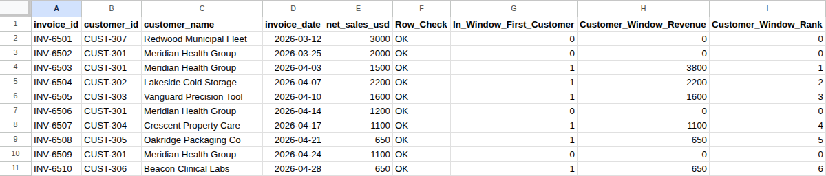
Create a tab called Customer_Revenue. Put the headings invoice_id, customer_id, customer_name, invoice_date, and net_sales_usd in A1:E1, and the ten invoices in rows 2 to 11. Enter the dates as real dates, not text.
| Row | invoice_id (A) | customer_id (B) | customer_name (C) | invoice_date (D) | net_sales_usd (E) |
|---|---|---|---|---|---|
| 2 | INV-6501 | CUST-307 | Redwood Municipal Fleet | 2026-03-12 | 3000 |
| 3 | INV-6502 | CUST-301 | Meridian Health Group | 2026-03-25 | 2000 |
| 4 | INV-6503 | CUST-301 | Meridian Health Group | 2026-04-03 | 1500 |
| 5 | INV-6504 | CUST-302 | Lakeside Cold Storage | 2026-04-07 | 2200 |
| 6 | INV-6505 | CUST-303 | Vanguard Precision Tool | 2026-04-10 | 1600 |
| 7 | INV-6506 | CUST-301 | Meridian Health Group | 2026-04-14 | 1200 |
| 8 | INV-6507 | CUST-304 | Crescent Property Care | 2026-04-17 | 1100 |
| 9 | INV-6508 | CUST-305 | Oakridge Packaging Co | 2026-04-21 | 650 |
| 10 | INV-6509 | CUST-301 | Meridian Health Group | 2026-04-24 | 1100 |
| 11 | INV-6510 | CUST-306 | Beacon Clinical Labs | 2026-04-28 | 650 |
Before using your own export, check four things:
- One row per invoice. Some exports list each line item on its own row. Collapse those to one row per invoice. Duplicate sales rows or legitimate order lines? shows how to tell the difference.
- Positive invoices only. This version isn’t built for credit memos, refunds, or zero-dollar invoices. If your export has them, stop here. Don’t delete credits to pass the check, because the total would then overstate net sales.
- Whole cents. Each stored amount must be at least $0.01, with no more than two decimal places. Formatting a cell to show cents doesn’t round the stored value. A hidden fraction of a cent can make the reconciliation stop, or show
#DIV/0!in L9 and L11. - Dates without times. If a date carries a time, such as 2026-04-28 14:22, convert it to a whole date with
INT.
Put Row_Check in F1. Enter this in F2 and copy it down to F11:
=IF(OR(COUNTA(A2:E2)<5, NOT(ISTEXT(A2)), NOT(ISTEXT(B2)), NOT(ISTEXT(C2)), TRIM(SUBSTITUTE(A2, CHAR(160), " "))="", TRIM(SUBSTITUTE(B2, CHAR(160), " "))="", TRIM(SUBSTITUTE(C2, CHAR(160), " "))="", NOT(EXACT(A2, TRIM(SUBSTITUTE(A2, CHAR(160), " ")))), NOT(EXACT(B2, TRIM(SUBSTITUTE(B2, CHAR(160), " ")))), NOT(EXACT(C2, TRIM(SUBSTITUTE(C2, CHAR(160), " ")))), LEN(A2)<>8, NOT(EXACT(LEFT(A2, 4), "INV-")), NOT(ISNUMBER(FIND(MID(A2, 5, 1), "0123456789"))), NOT(ISNUMBER(FIND(MID(A2, 6, 1), "0123456789"))), NOT(ISNUMBER(FIND(MID(A2, 7, 1), "0123456789"))), NOT(ISNUMBER(FIND(MID(A2, 8, 1), "0123456789"))), LEN(B2)<>8, NOT(EXACT(LEFT(B2, 5), "CUST-")), NOT(ISNUMBER(FIND(MID(B2, 6, 1), "0123456789"))), NOT(ISNUMBER(FIND(MID(B2, 7, 1), "0123456789"))), NOT(ISNUMBER(FIND(MID(B2, 8, 1), "0123456789"))), NOT(ISNUMBER(D2)), NOT(ISNUMBER(E2))), "CHECK INPUTS", IF(OR(D2<DATE(2000,1,1), INT(D2)<>D2, E2<=0, SUMPRODUCT(--(UPPER($A$2:$A$11)=UPPER(A2)))>1, SUMPRODUCT(--EXACT($B$2:$B$11, B2), --NOT(EXACT($C$2:$C$11, C2)))>0, SUMPRODUCT(--(UPPER($C$2:$C$11)=UPPER(C2)), --NOT(EXACT($B$2:$B$11, B2)))>0), "CHECK INPUTS", "OK"))
All ten rows should say OK. A row returns CHECK INPUTS if any of these is true:
- A cell is blank, or has extra or non-breaking spaces.
- An ID doesn’t follow this example’s INV- plus four digits or CUST- plus three digits format.
- The date is text, has a time attached, or is before 2000.
- The amount is zero or negative.
- The invoice ID appears twice. An uncollapsed line-item export fails here.
- One customer ID has two names, or one name (ignoring case) has two customer IDs.
The check only catches conflicts it can see. If one company sits under a second ID and a slightly different name, every row passes. Put INV-6506 and INV-6509 under CUST-308 "Meridian Health" on a copy: the top customer drops to $2,300 (23%), and the sheet still reconciles. Scan your customer list for duplicate accounts before ranking. Find unmatched customer IDs with XLOOKUP helps with the ID side.
Step 2: Roll Up Each Customer and Rank Them
Set the window first. Put Check_Item, Window_Customer_Benchmark, and Candidate_KPI_Audit in K1:M1. In K2:K14, enter Concentration_Scope, Window_Start, Window_End, Window_Invoice_Rows, Window_Net_Sales_USD, Distinct_Active_Customers, Top_1_Customer_Revenue_USD, Top_1_Customer_Share, Top_5_Customer_Revenue_USD, Top_5_Customer_Share, Rollup_And_Top_Revenue_Gap_USD, Share_Gap_Percentage_Points, and Reconciliation_Status. Then set L2 = CUSTOMER_WINDOW, L3 = 2026-04-01, and L4 = 2026-04-30, as real dates. Set M2 = NOT TESTED and leave M3:M11 blank.
Put In_Window_First_Customer in G1. In G2, copied down to G11:
=IF(OR(NOT(EXACT(F2, "OK")), COUNTIF($F$2:$F$11, "OK")<10, NOT(ISNUMBER($L$3)), NOT(ISNUMBER($L$4))), "CHECK INPUTS", IF(OR($L$3<DATE(2000,1,1), INT($L$3)<>$L$3, $L$4<DATE(2000,1,1), INT($L$4)<>$L$4, $L$4<$L$3), "CHECK INPUTS", IF(AND(D2>=$L$3, D2<=$L$4, SUMPRODUCT(--EXACT($B$2:B2, B2), --($D$2:D2>=$L$3), --($D$2:D2<=$L$4))=1), 1, 0)))
The range $B$2:B2 grows as you copy it down, so each row looks only at itself and the rows above. A row gets a 1 when it’s inside the window and is that customer’s first in-window invoice. Meridian’s 1 lands on row 4.
Put Customer_Window_Revenue in H1. In H2, copied down to H11:
=IF(OR(NOT(ISNUMBER(G2)), COUNT($G$2:$G$11)<10), "CHECK INPUTS", IF(G2=1, ROUND(SUMPRODUCT(--EXACT($B$2:$B$11, B2), --($D$2:$D$11>=$L$3), --($D$2:$D$11<=$L$4), $E$2:$E$11), 2), 0))
H puts each customer’s window total on its flagged row and 0 elsewhere, so column H adds up to April sales with no customer counted twice.
Put Customer_Window_Rank in I1. In I2, copied down to I11:
=IF(OR(NOT(ISNUMBER(H2)), COUNT($H$2:$H$11)<10), "CHECK INPUTS", IF(G2=1, SUMPRODUCT(--($G$2:$G$11=1), --($H$2:$H$11>H2)) + SUMPRODUCT(--($G$2:G2=1), --($H$2:H2=H2)), 0))
The first part counts customers with higher totals. The second breaks exact ties by row order, so every active customer gets a different rank from 1 to 6.
| Row | invoice_id | customer_id | G | H | I |
|---|---|---|---|---|---|
| 2–3 | INV-6501, INV-6502 | (March) | 0 | 0 | 0 |
| 4 | INV-6503 | CUST-301 | 1 | 3800 | 1 |
| 5 | INV-6504 | CUST-302 | 1 | 2200 | 2 |
| 6 | INV-6505 | CUST-303 | 1 | 1600 | 3 |
| 7 | INV-6506 | CUST-301 | 0 | 0 | 0 |
| 8 | INV-6507 | CUST-304 | 1 | 1100 | 4 |
| 9 | INV-6508 | CUST-305 | 1 | 650 | 5 |
| 10 | INV-6509 | CUST-301 | 0 | 0 | 0 |
| 11 | INV-6510 | CUST-306 | 1 | 650 | 6 |
If you sort the export newest first, Beacon takes rank 5 and Oakridge rank 6. The Top-5 total doesn’t change.
The matching uses SUMPRODUCT with EXACT, not COUNTIFS. COUNTIF is not case-sensitive and treats ? and * as wildcards, so it can match IDs that aren’t the same. EXACT compares every character. The COUNTIF on column F is safe, because it looks for the fixed word OK.
Step 3: Build the Reconciliation Block
Column L is the benchmark. In L5:
=IF(OR(NOT(EXACT(L2, "CUSTOMER_WINDOW")), NOT(ISNUMBER(L3)), NOT(ISNUMBER(L4)), COUNTIF($F$2:$F$11, "OK")<10, COUNT($G$2:$G$11)<10, COUNT($H$2:$H$11)<10, COUNT($I$2:$I$11)<10), "CHECK INPUTS", IF(OR(L3<DATE(2000,1,1), INT(L3)<>L3, L4<DATE(2000,1,1), INT(L4)<>L4, L4<L3, SUM($G$2:$G$11)<5), "CHECK INPUTS", SUMPRODUCT(--($D$2:$D$11>=L3), --($D$2:$D$11<=L4))))
L5 also stops the sheet if the window has fewer than five active customers. That’s this sheet’s rule, so the Top-5 figure is never padded with empty rows. With exactly five customers, Top-5 is always 100%, which tells you little.
Then L6 to L13:
- L6:
=IF(NOT(ISNUMBER(L5)), "CHECK INPUTS", ROUND(SUMPRODUCT(--($D$2:$D$11>=L3), --($D$2:$D$11<=L4), $E$2:$E$11), 2)) - L7:
=IF(NOT(ISNUMBER(L5)), "CHECK INPUTS", SUM($G$2:$G$11)) - L8:
=IF(NOT(ISNUMBER(L5)), "CHECK INPUTS", ROUND(SUMPRODUCT(--($I$2:$I$11=1), $H$2:$H$11), 2)) - L9:
=IF(NOT(ISNUMBER(L5)), "CHECK INPUTS", ROUND(L8/L6, 4)) - L10:
=IF(NOT(ISNUMBER(L5)), "CHECK INPUTS", ROUND(SUMPRODUCT(--($I$2:$I$11>=1), --($I$2:$I$11<=5), $H$2:$H$11), 2)) - L11:
=IF(NOT(ISNUMBER(L5)), "CHECK INPUTS", ROUND(L10/L6, 4)) - L12:
=IF(NOT(ISNUMBER(L5)), "CHECK INPUTS", ROUND(ABS(L6-SUM($H$2:$H$11)) + ABS(L8-LARGE($H$2:$H$11, 1)) + ABS(L10-(LARGE($H$2:$H$11, 1)+LARGE($H$2:$H$11, 2)+LARGE($H$2:$H$11, 3)+LARGE($H$2:$H$11, 4)+LARGE($H$2:$H$11, 5))), 2)) - L13:
=IF(NOT(ISNUMBER(L5)), "CHECK INPUTS", 0)
L12 checks the rollup three ways. Column H must total window sales, L8 must equal the largest value in H, and L10 must equal the five largest values added up. So the rank-based Top-1 and Top-5 amounts must agree with LARGE, which doesn’t use the rank column. L13 is a zero that keeps the rows lined up with column M. L14 writes the status:
=IF(OR(NOT(ISNUMBER(L5)), NOT(ISNUMBER(L6)), NOT(ISNUMBER(L7)), NOT(ISNUMBER(L8)), NOT(ISNUMBER(L9)), NOT(ISNUMBER(L10)), NOT(ISNUMBER(L11)), NOT(ISNUMBER(L12)), NOT(ISNUMBER(L13))), "CHECK INPUTS", IF(OR(L12<>0, L13<>0, L8<=0, L10<L8, L10>L6), "CHECK INPUTS", "RECONCILED: TOP-1 " & TEXT(L9, "0.00%") & " ($" & TEXT(L8, "0.00") & ") / TOP-5 " & TEXT(L11, "0.00%") & " ($" & TEXT(L10, "0.00") & ") OF $" & TEXT(L6, "0.00") & " (" & L7 & " CUSTOMERS)"))
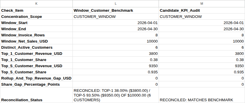
L14 should read RECONCILED: TOP-1 38.00% ($3800.00) / TOP-5 93.50% ($9350.00) OF $10000.00 (6 CUSTOMERS).
To see the window effect, set L3 to 2026-03-01. L14 changes to RECONCILED: TOP-1 38.67% ($5800.00) / TOP-5 91.33% ($13700.00) OF $15000.00 (7 CUSTOMERS). Set L4 to 2026-03-31 as well, and only two customers remain, so L14 says CHECK INPUTS. Set L3 back to 2026-04-01 and L4 back to 2026-04-30 before going on.
Column M audits a reported number, such as a dashboard card. After the three formulas below are in, you’ll enter CUSTOMER_WINDOW in M2, the window in M3:M4 as real dates, and the reported figures in M5:M11. Type shares as decimals: 0.38, not 38. In M12:
=IF(OR(EXACT(L14, "CHECK INPUTS"), NOT(OR(M2="", EXACT(M2, "NOT TESTED"), EXACT(M2, "CUSTOMER_WINDOW"))), IF(ISNUMBER(M3), OR(M3<DATE(2000,1,1), INT(M3)<>M3), NOT(OR(M3="", EXACT(M3, "NOT TESTED")))), IF(ISNUMBER(M4), OR(M4<DATE(2000,1,1), INT(M4)<>M4), NOT(OR(M4="", EXACT(M4, "NOT TESTED")))), IF(AND(ISNUMBER(M3), ISNUMBER(M4)), M4<M3, FALSE), IF(ISNUMBER(M5), OR(M5<=0, INT(M5)<>M5), NOT(OR(M5="", EXACT(M5, "NOT TESTED")))), IF(ISNUMBER(M6), M6<=0, NOT(OR(M6="", EXACT(M6, "NOT TESTED")))), IF(ISNUMBER(M7), OR(M7<=0, INT(M7)<>M7), NOT(OR(M7="", EXACT(M7, "NOT TESTED")))), IF(ISNUMBER(M8), M8<=0, NOT(OR(M8="", EXACT(M8, "NOT TESTED")))), IF(ISNUMBER(M9), OR(M9<=0, M9>1), NOT(OR(M9="", EXACT(M9, "NOT TESTED")))), IF(ISNUMBER(M10), M10<=0, NOT(OR(M10="", EXACT(M10, "NOT TESTED")))), IF(ISNUMBER(M11), OR(M11<=0, M11>1), NOT(OR(M11="", EXACT(M11, "NOT TESTED")))), IF(AND(ISNUMBER(M8), ISNUMBER(M10)), M10<M8, FALSE), IF(AND(ISNUMBER(M9), ISNUMBER(M11)), M11<M9, FALSE)), "CHECK INPUTS", IF(OR(M2="", EXACT(M2, "NOT TESTED"), NOT(ISNUMBER(M3)), NOT(ISNUMBER(M4)), NOT(ISNUMBER(M5)), NOT(ISNUMBER(M6)), NOT(ISNUMBER(M7)), NOT(ISNUMBER(M8)), NOT(ISNUMBER(M9)), NOT(ISNUMBER(M10)), NOT(ISNUMBER(M11))), "NOT TESTED", ROUND(ABS(M6-L6) + ABS(M8-L8) + ABS(M10-L10), 2)))
M13 adds up the share differences in percentage points:
=IF(EXACT(M12, "CHECK INPUTS"), "CHECK INPUTS", IF(EXACT(M12, "NOT TESTED"), "NOT TESTED", ROUND((ABS(M9-L9) + ABS(M11-L11))*100, 2)))
M14 checks the window first, then the customer count, then Top-1, then Top-5:
=IF(OR(EXACT(M12, "CHECK INPUTS"), EXACT(M13, "CHECK INPUTS")), "CHECK INPUTS", IF(OR(EXACT(M12, "NOT TESTED"), EXACT(M13, "NOT TESTED")), "NOT TESTED: ENTER CANDIDATE KPI VALUES", IF(OR(M3<>L3, M4<>L4, M5<>L5, ROUND(M6-L6, 2)<>0), "STOP: WINDOW BOUNDARY MISMATCH (CHECK START/END DATES)", IF(M7<>L7, "STOP: CUSTOMER GRAIN MISMATCH (AGGREGATE BY CUSTOMER ID NOT INVOICE ROWS)", IF(OR(ROUND(M8-L8, 2)<>0, ROUND(M9-L9, 4)<>0, ROUND(M9-ROUND(M8/M6, 4), 4)<>0), "STOP: TOP-1 CUSTOMER SHARE MISMATCH (SUM ALL INVOICES PER CUSTOMER)", IF(OR(ROUND(M10-L10, 2)<>0, ROUND(M11-L11, 4)<>0, ROUND(M11-ROUND(M10/M6, 4), 4)<>0, M12<>0, M13<>0), "STOP: TOP-5 CUSTOMER SHARE MISMATCH (CHECK TIE HANDLING AND 5-CUSTOMER SUM)", "RECONCILED: MATCHES BENCHMARK"))))))
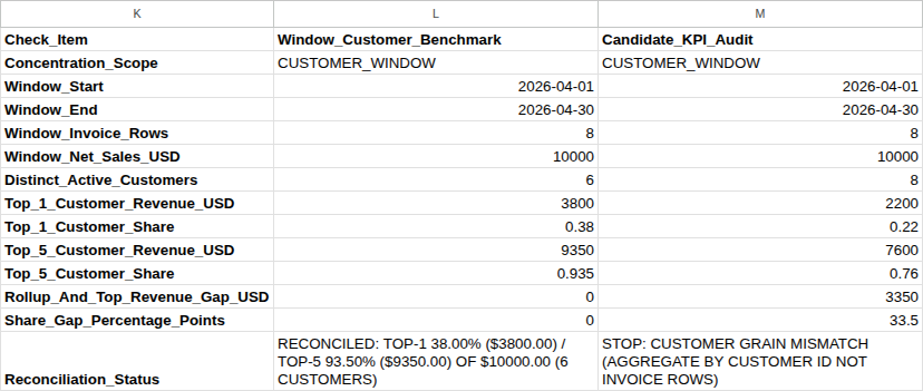
With M2 still NOT TESTED, M14 says NOT TESTED: ENTER CANDIDATE KPI VALUES. Now enter each row below into M2:M11, with CUSTOMER_WINDOW in M2. Fill in every cell for each test. Trap 1 starts at the first invoice in the export, so it uses M3 = 2026-03-12, M4 = 2026-04-30, M5 = 10, and M6 = 15000. Every other test uses M3 = 2026-04-01, M4 = 2026-04-30, M5 = 8, and M6 = 10000.
| Test | M3:M6 | M7 | M8 | M9 | M10 | M11 | M12 | M13 | M14 result (shortened) |
|---|---|---|---|---|---|---|---|---|---|
| Trap 1 | Mar 12 to Apr 30, 10, 15000 | 7 | 5800 | 0.3867 | 13700 | 0.9133 | 11350 | 2.84 | STOP: WINDOW BOUNDARY MISMATCH |
| Trap 2 | Apr 1 to Apr 30, 8, 10000 | 8 | 2200 | 0.22 | 7600 | 0.76 | 3350 | 33.5 | STOP: CUSTOMER GRAIN MISMATCH |
| Trap 3 | Apr 1 to Apr 30, 8, 10000 | 6 | 2200 | 0.22 | 9350 | 0.935 | 1600 | 16 | STOP: TOP-1 CUSTOMER SHARE MISMATCH |
| Trap 4 | Apr 1 to Apr 30, 8, 10000 | 6 | 3800 | 0.38 | 10000 | 1 | 650 | 6.5 | STOP: TOP-5 CUSTOMER SHARE MISMATCH |
| Correct | Apr 1 to Apr 30, 8, 10000 | 6 | 3800 | 0.38 | 9350 | 0.935 | 0 | 0 | RECONCILED: MATCHES BENCHMARK |
The full STOP messages are in the M14 formula. M12 and M13 add up several separate differences, so read them as "how far off," not as missing dollars or a single change in share. The customer-count message names invoice rows as the cause because that’s the usual one. It also fires if a report counts a customer with no sales in the window.
With the correct values entered, try typing 93.5 instead of 0.935 in M11. Column M returns CHECK INPUTS, and L14 stays reconciled. Change M11 back to 0.935 when you’re done.
Adapting the Sheet to Your Own Export
These formulas are written for ten invoices. For your file:
- Copy F2:I2 down to your last invoice row. Extend every fixed range,
$A$2:$A$11through$I$2:$I$11, to that row, in columns F to I and in L5:L12. A range left ending at row 11 drops the rows below it from the totals, and nothing warns you. The growing ranges in G2 and I2 ($B$2:B2,$D$2:D2,$G$2:G2,$H$2:H2) stay anchored at row 2 and extend on their own. - Replace the 10 in each row-count check with your number of invoice rows. There are seven:
COUNTIF($F$2:$F$11, "OK")<10in G2 and L5,COUNT($G$2:$G$11)<10in H2 and L5,COUNT($H$2:$H$11)<10in I2 and L5, andCOUNT($I$2:$I$11)<10in L5. Left at 10, they stop a shorter file withCHECK INPUTSand don’t fully check a longer one. Don’t use find-and-replace on 10 or 11: L10, L11, M10, M11, and the 100 in M13 contain the same digits. - Change or remove the INV- and CUST- format checks in F2 to match your billing system’s IDs.
Checklist Before You Share the Numbers
- F2:F11 all say
OK, and every amount is a positive, whole-cent invoice. - Column H adds up to window sales, and L12 is 0.
- Top-1 and Top-5 come from customer totals in column H, not from invoice amounts in column E.
- Any tie at fifth place, or at first, is disclosed next to the names.
- The report header states the window dates and that the figures are invoiced net sales. Duplicate customer accounts were checked first.
What to Do Next
If a dashboard’s concentration figure still doesn’t match, why the dashboard total differs from the spreadsheet walks through the same kind of reconciliation for totals. If customer names and IDs in your export are messy, start with a repeatable workflow for cleaning business spreadsheet data.