
To find unmatched customer IDs, give XLOOKUP an explicit label for missing matches: =XLOOKUP(B2, Customers!$A$2:$A$6, Customers!$C$2:$C$6, "UNMATCHED ID", 0). Don’t use "" or 0 there, or wrap the formula in IFERROR. A SUMIFS report by segment then drops those rows without showing an error. Next, work out why each ID failed, and approve the report only when both the unmatched dollars and the unmatched row count are zero.
How $3,300 Disappears
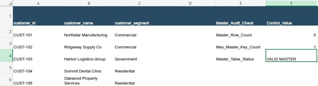
Here’s a made-up example: a Customers tab with five customers and an Invoices tab with seven April invoices totaling $8,400. On Customers, put the headings customer_id, customer_name, and customer_segment in A1:C1 and these rows below:
| Row | customer_id (A) | customer_name (B) | customer_segment (C) |
|---|---|---|---|
| 2 | CUST-101 | Northstar Manufacturing | Commercial |
| 3 | CUST-102 | Ridgeway Supply Co | Commercial |
| 4 | CUST-103 | Harbor Logistics Group | Government |
| 5 | CUST-104 | Summit Dental Clinic | Residential |
| 6 | CUST-105 | Oakwood Property Services | Residential |
On Invoices, put invoice_id, customer_id_raw, invoice_date, and invoice_amount in A1:D1. Type the dates as real dates and the amounts as plain numbers:
| Row | invoice_id (A) | customer_id_raw (B) | invoice_date (C) | invoice_amount (D) |
|---|---|---|---|---|
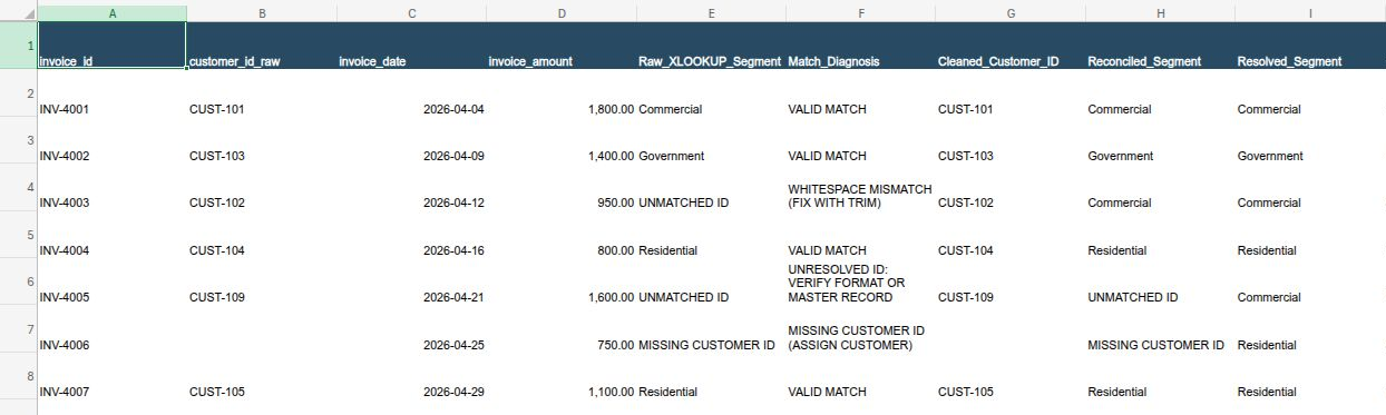
| 2 | INV-4001 | CUST-101 | 2026-04-04 | 1800 |
| 3 | INV-4002 | CUST-103 | 2026-04-09 | 1400 |
| 4 | INV-4003 | CUST-102 (one trailing space) |
2026-04-12 | 950 |
| 5 | INV-4004 | CUST-104 | 2026-04-16 | 800 |
| 6 | INV-4005 | CUST-109 | 2026-04-21 | 1600 |
| 7 | INV-4006 | (leave blank) | 2026-04-25 | 750 |
| 8 | INV-4007 | CUST-105 | 2026-04-29 | 1100 |
The space after CUST-102 in B4 is deliberate. =LEN(B4) should return 9. Four invoices match cleanly. Three don’t: row 4 has the trailing space, row 6’s CUST-109 isn’t in the customer list, and row 7 has no customer ID at all.
If the lookup returns "" for those rows, a SUMIFS report of the three segments shows $5,100. That leaves out $3,300, or 39.29% of the month’s revenue, and every cell on the page looks fine. A blank fallback is harmless in a notes column. In any column that a SUMIFS or pivot table summarizes, a failed lookup is an exception and needs a label.
Step 1: Check the Customer List First
A lookup is only as good as the list it reads. On the Customers tab, put the labels Master_Audit_Check, Master_Row_Count, Max_Master_Key_Count, and Master_Table_Status in E1:E4, and Control_Value in F1. Then in F2:
=COUNTA(A2:A6)
In F3, which checks that every row is filled in with no stray spaces, then returns the most times any ID appears:
=IF(OR(COUNTA(A2:A6)<5, COUNTA(B2:B6)<5, COUNTA(C2:C6)<5, SUMPRODUCT(--(A2:A6<>TRIM(A2:A6)))>0, SUMPRODUCT(--(B2:B6<>TRIM(B2:B6)))>0), "CHECK MASTER", MAX(COUNTIF(A2:A6, A2:A6)))
In F4:
=IF(NOT(ISNUMBER(F3)), "CHECK MASTER", IF(OR(F3>1, COUNTIF(C2:C6, "Commercial")+COUNTIF(C2:C6, "Government")+COUNTIF(C2:C6, "Residential")<>COUNTA(A2:A6)), "CHECK MASTER", "VALID MASTER"))
F4 should say VALID MASTER: five complete rows, no ID listed twice, and every segment one of the three allowed names. The checks don’t confirm that each ID follows your format, such as CUST- plus three digits. If the format matters, enforce it where IDs are created.
Step 2: Look Up With an Explicit Flag (Column E)
On Invoices, put the heading Raw_XLOOKUP_Segment in E1, enter this in E2, and copy it down to E8:
=IF(OR(TRIM(A2)="", NOT(ISNUMBER(C2)), NOT(ISNUMBER(D2)), ISNUMBER(FIND("*", B2)), ISNUMBER(FIND("?", B2)), ISNUMBER(FIND("~", B2))), "CHECK INPUTS", IF(OR(C2<DATE(2000,1,1), D2<0), "CHECK INPUTS", IF(TRIM(SUBSTITUTE(B2, CHAR(160), " "))="", "MISSING CUSTOMER ID", XLOOKUP(B2, Customers!$A$2:$A$6, Customers!$C$2:$C$6, "UNMATCHED ID", 0))))
The first IF confirms there’s an invoice ID, a date stored as a number, and a numeric amount, and that the customer ID contains no *, ?, or ~. Only then does the second IF compare the date and amount, so a "TBD" never causes an error. A blank ID, or one made only of spaces, is labeled MISSING CUSTOMER ID. Everything else goes to XLOOKUP, which returns the segment or UNMATCHED ID.
The wildcard check matters for the next step. XLOOKUP’s exact match treats * literally, but MATCH with a match type of 0 treats * and ? as wildcards, so an ID like CUST-10* could falsely match CUST-101.
XLOOKUP’s exact match ignores capitalization, so cust-101 finds CUST-101. It doesn’t ignore a trailing space, a non-breaking space, or a number stored where the list holds text. Two IDs that look the same on screen can still fail.
Step 3: Diagnose Each Failure (Column F)
The tempting rule is "if it still fails after TRIM, add it to the customer list." That can create a duplicate customer. Put Match_Diagnosis in F1, enter this in F2, and copy it to F8:
=IF(E2="CHECK INPUTS", "CHECK INPUTS", IF(E2="MISSING CUSTOMER ID", "MISSING CUSTOMER ID (ASSIGN CUSTOMER)", IF(E2<>"UNMATCHED ID", "VALID MATCH", IF(ISNUMBER(B2), "TYPE MISMATCH: NUMBER VS TEXT ID", IF(ISNUMBER(MATCH(TRIM(B2), Customers!$A$2:$A$6, 0)), "WHITESPACE MISMATCH (FIX WITH TRIM)", IF(ISNUMBER(MATCH(TRIM(SUBSTITUTE(B2, CHAR(160), " ")), Customers!$A$2:$A$6, 0)), "NBSP CHAR(160) MISMATCH (CLEAN WITH SUBSTITUTE+TRIM)", "UNRESOLVED ID: VERIFY FORMAT OR MASTER RECORD"))))))
For each unmatched ID, it asks in order:
- Is it a number? An ID typed as 104 won’t match text. This check runs before TRIM, because TRIM turns a number into text, which would make a type problem look like a spacing problem.
- Does it match after removing spaces? Row 4’s
CUST-102does, so F4 saysWHITESPACE MISMATCH (FIX WITH TRIM). - Does it match after converting non-breaking spaces? TRIM doesn’t remove CHAR(160), the non-breaking space that often comes along when text is copied from a web page. SUBSTITUTE turns it into an ordinary space first.
- Otherwise, the label says to verify the format or the customer record. Row 6’s CUST-109 lands here. Check the source system before you add anyone.
Step 4: Clean the IDs and Look Up Again (Columns G and H)
Put Cleaned_Customer_ID in G1 and Reconciled_Segment in H1. In G2, copied to G8:
=IF(E2="CHECK INPUTS", "CHECK INPUTS", IF(ISNUMBER(B2), B2, TRIM(SUBSTITUTE(B2, CHAR(160), " "))))
In H2, copied to H8:
=IF(E2="CHECK INPUTS", "CHECK INPUTS", IF(G2="", "MISSING CUSTOMER ID", XLOOKUP(G2, Customers!$A$2:$A$6, Customers!$C$2:$C$6, "UNMATCHED ID", 0)))
Row 4 now finds CUST-102 and returns Commercial, recovering $950. The raw ID in column B stays as it was. Numeric IDs pass through unchanged on purpose. Whether 104 means CUST-104 or "0104" depends on your ID standard, so investigate those rows instead of guessing. Build a small data dictionary for your spreadsheet covers writing that standard down.
Step 5: Reconcile Rows and Dollars (J1:N10)
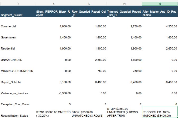
Next to the invoices, build a reconciliation block. Put Segment_Bucket in J1 and these labels in J2:J10: Commercial, Government, Residential, UNMATCHED ID, MISSING CUSTOMER ID, Report_Subtotal, Variance_vs_Invoices, Exception_Row_Count, Reconciliation_Status.
Column L summarizes the raw lookup in column E, and column M the cleaned lookup in column H. Put Raw_Guarded_Report in L1 and Trimmed_Guarded_Report in M1. The rest of the formulas, including the optional column K and the resolved column N, are in the reference section at the end. In L2, copied to L6:
=IF(OR(Customers!$F$4<>"VALID MASTER", COUNTA($A$2:$A$8)<7, COUNT($D$2:$D$8)<>COUNTA($A$2:$A$8), COUNTIF($E$2:$E$8, "CHECK INPUTS")>0), "CHECK INPUTS", SUMIFS($D$2:$D$8, $E$2:$E$8, $J2))
Then copy L7:L10 across to M7:M10:
- L7:
=IF(COUNT(L2:L6)<5, "CHECK INPUTS", SUM(L2:L6)) - L8:
=IF(NOT(ISNUMBER(L7)), "CHECK INPUTS", ROUND(L7 - SUM($D$2:$D$8), 2)) - L9:
=IF(NOT(ISNUMBER(L8)), "CHECK INPUTS", COUNTA($A$2:$A$8) - (COUNTIF($E$2:$E$8, $J$2) + COUNTIF($E$2:$E$8, $J$3) + COUNTIF($E$2:$E$8, $J$4)))
L10:
=IF(NOT(ISNUMBER(L9)), "CHECK INPUTS", IF(L8<>0, "STOP: $" & TEXT(ABS(L8), "0.00") & " OMITTED (" & TEXT(L8/SUM($D$2:$D$8), "0.00%") & ")", IF(OR(ROUND(L5+L6, 2)>0, L9>0), "STOP: $" & TEXT(L5+L6, "0.00") & " UNMATCHED (" & L9 & " ROWS)", "RECONCILED: 100% MATCHED ($" & TEXT(L7, "0.00") & ")")))
In column M, change $E$2:$E$8 to $H$2:$H$8 in M2:M6 and M9. Add COUNTIF($H$2:$H$8, "CHECK INPUTS")>0 to the M2 guard. Then add " AFTER TRIM" to M10’s label.
| Silent report (K) | Raw lookup (L) | After cleanup (M) | After resolution (N) | |
|---|---|---|---|---|
| Commercial | $1,800 | $1,800 | $2,750 | $4,350 |
| Government | $1,400 | $1,400 | $1,400 | $1,400 |
| Residential | $1,900 | $1,900 | $1,900 | $2,650 |
| UNMATCHED ID | $0 | $2,550 | $1,600 | $0 |
| MISSING CUSTOMER ID | $0 | $750 | $750 | $0 |
| Subtotal | $5,100 | $8,400 | $8,400 | $8,400 |
| Exception rows | 3 | 3 | 2 | 0 |
| Status | STOP: $3300.00 OMITTED (-39.29%) | STOP: $3300.00 UNMATCHED (3 ROWS) | STOP: $2350.00 UNMATCHED (2 ROWS AFTER TRIM) | RECONCILED: 100% MATCHED ($8400.00) |
Columns L and M both add up to $8,400, with no variance, and still refuse to approve, because money sits in the exception rows. The row count matters too. On a copy, set the amounts in D4, D6, and D7 to zero: the exception dollars become $0.00, yet L10 still says STOP: $0.00 UNMATCHED (3 ROWS). A zero-dollar credit memo with an unknown customer is still unattributed. Restore the original amounts ($950, $1,600, and $750) before you go on.
A labeled fallback doesn’t fix the segment totals by itself. SUMIFS over Commercial, Government, and Residential leaves the exception rows out whether the fallback is blank or UNMATCHED ID. What makes the omission visible is the two exception buckets in rows 5 and 6 and the row count in row 9.
Step 6: Resolve the Rest Without Overwriting the Source
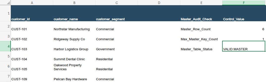
Suppose that, in this example, the billing system confirms CUST-109 is a new customer, Pelican Bay Hardware, Commercial. It also shows that INV-4006 belongs to CUST-104, Summit Dental Clinic, Residential.
Don’t edit the original tabs. Copy Customers to a new tab, Customers_Resolved, and add CUST-109 in row 7. Change its control formulas to cover rows 2 to 7 and expect 6 rows. Then put Resolved_Segment in I1 and enter this in I2, copied to I8:
=IF(OR(E2="CHECK INPUTS", Customers_Resolved!$F$4<>"VALID MASTER"), "CHECK INPUTS", IF(IF(A2="INV-4006", "CUST-104", G2)="", "MISSING CUSTOMER ID", XLOOKUP(IF(A2="INV-4006", "CUST-104", G2), Customers_Resolved!$A$2:$A$7, Customers_Resolved!$C$2:$C$7, "UNMATCHED ID", 0)))
The INV-4006 override applies to this one verified invoice only. It isn’t a rule for other imports. The order of checks matters: the outer IF checks the row’s inputs and the resolved list before the override runs. If INV-4006 had a "TBD" date or an invalid amount, column I would still show CHECK INPUTS instead of quietly returning Residential.
Column N, built from column I (see the reference section), shows all seven invoices matched, $8,400, and RECONCILED. These ranges are fixed at five or six customers and seven invoices. Extend every one of them when your data grows.
Troubleshooting
| Symptom | Cause | Fix |
|---|---|---|
| Every report column says CHECK INPUTS | A blank invoice ID, a text or pre-2000 date, a text or negative amount, a wildcard in an ID, or F4 isn’t VALID MASTER | Fix the flagged row or the customer list |
| Report short by exactly the unmatched rows | Blank or zero fallback in XLOOKUP | Use "UNMATCHED ID" and include the exception buckets |
| TYPE MISMATCH in column F | The ID was imported as a number | Re-import the column as text; check your ID standard |
| XLOOKUP returns #VALUE! | Lookup and return ranges differ in height | Make both ranges the same height |
Frequently Asked Questions
What if a customer ID appears twice in the list?
XLOOKUP returns the first match and ignores the rest, so if the two rows list different segments, the lookup can pull the wrong one without warning. That’s why F3 counts how often each ID appears, and F4 blocks the report when any ID appears more than once.
What to Do Next
If IDs lose their format on the way in, start with import a CSV into Excel without losing leading zeros. For the full cleanup routine, see a repeatable workflow for cleaning business spreadsheet data. The reconciliation block is one item in The Small Business Data Audit Checklist.
Copy-Paste Formula Reference
Column K (optional, the silent report). K2:K4 use the L2 formula. K5 and K6 hold =IF(NOT(ISNUMBER(K2)), "CHECK INPUTS", 0), standing in for exception rows the report never shows. K7:K10 are copied from L7:L10.
M2, copied to M6:
=IF(OR(Customers!$F$4<>"VALID MASTER", COUNTA($A$2:$A$8)<7, COUNT($D$2:$D$8)<>COUNTA($A$2:$A$8), COUNTIF($E$2:$E$8, "CHECK INPUTS")>0, COUNTIF($H$2:$H$8, "CHECK INPUTS")>0), "CHECK INPUTS", SUMIFS($D$2:$D$8, $H$2:$H$8, $J2))
M9: =IF(NOT(ISNUMBER(M8)), "CHECK INPUTS", COUNTA($A$2:$A$8) - (COUNTIF($H$2:$H$8, $J$2) + COUNTIF($H$2:$H$8, $J$3) + COUNTIF($H$2:$H$8, $J$4)))
M10:
=IF(NOT(ISNUMBER(M9)), "CHECK INPUTS", IF(M8<>0, "STOP: $" & TEXT(ABS(M8), "0.00") & " OMITTED (" & TEXT(M8/SUM($D$2:$D$8), "0.00%") & ")", IF(OR(ROUND(M5+M6, 2)>0, M9>0), "STOP: $" & TEXT(M5+M6, "0.00") & " UNMATCHED (" & M9 & " ROWS AFTER TRIM)", "RECONCILED: 100% MATCHED ($" & TEXT(M7, "0.00") & ")")))
N2, copied to N6:
=IF(OR(Customers_Resolved!$F$4<>"VALID MASTER", COUNTA($A$2:$A$8)<7, COUNT($D$2:$D$8)<>COUNTA($A$2:$A$8), COUNTIF($E$2:$E$8, "CHECK INPUTS")>0, COUNTIF($I$2:$I$8, "CHECK INPUTS")>0), "CHECK INPUTS", SUMIFS($D$2:$D$8, $I$2:$I$8, $J2))
N7, N8, and N10: copy from L7, L8, and L10. N9: the L9 formula with $I$2:$I$8 in place of $E$2:$E$8.
Customers_Resolved F2:F4: the Step 1 formulas with every 2:6 range changed to 2:7 and each <5 changed to <6.