
To fix date locale mismatches before building a monthly report, stop a US (MM/DD/YYYY) parser from auto-converting DD/MM/YYYY exports. When interpreted as MM/DD/YYYY, asymmetric days 1–12 can swap day and month, while days 13 to 31 stay text or return conversion errors and drop out of monthly totals. In Power Query, use Change Type > Using Locale… (Date, English (United Kingdom)). In Sheets or Excel, keep raw dates as text, convert with DATE, and reconcile.
Changing the display format after an automatic import never fixes a swapped date. If a US-locale sheet reads 04/03/2026 (4 March 2026) as April 3, 2026, the cell stores serial 46115 instead of March 4’s 46085. Reformatting as yyyy-mm-dd only displays 2026-04-03.
Why a DD/MM/YYYY Export Breaks Monthly Reports in Two Ways
Here is a made-up UK export with seven non-negative customer invoices (INV-5001 to INV-5007) totaling $9,200.00 across March 2026 ($4,700.00, 4 rows) and April 2026 ($4,500.00, 3 rows), where one row represents one invoice. Save these four columns as uk-invoices.csv:
invoice_id,customer_id,invoice_date_uk_raw,invoice_amount
INV-5001,CUST-201,04/03/2026,1500.00
INV-5002,CUST-202,09/03/2026,1200.00
INV-5003,CUST-203,18/03/2026,1100.00
INV-5004,CUST-201,25/03/2026,900.00
INV-5005,CUST-204,03/04/2026,1800.00
INV-5006,CUST-205,11/04/2026,1400.00
INV-5007,CUST-202,22/04/2026,1300.00
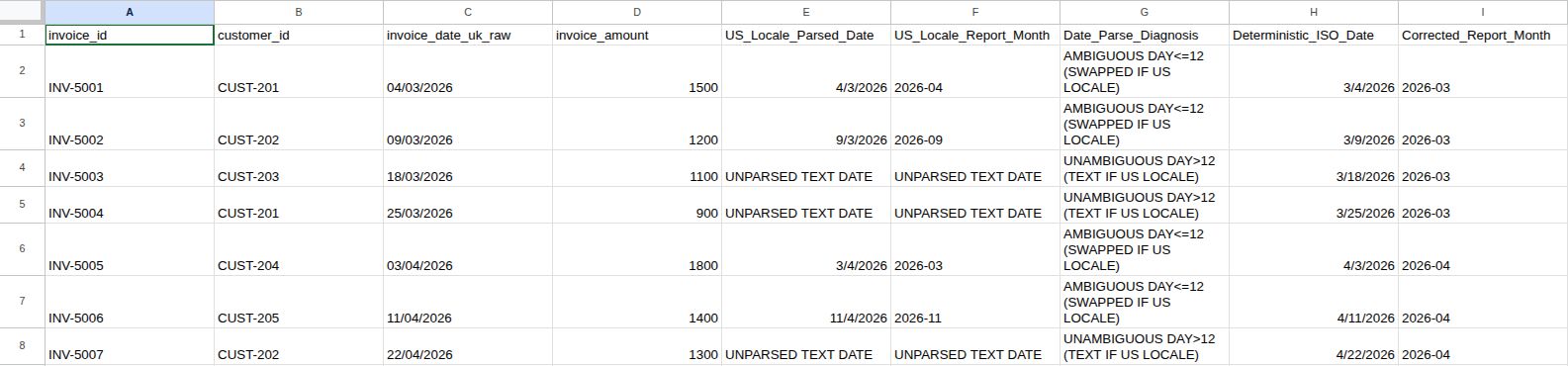
In Method 2, the four CSV columns sit in Raw_Export!A1:D8 and the calculated formulas sit in E1:I8 (Row is a row-number guide, not a column to paste):
| Row | A: invoice_id | B: customer_id | C: invoice_date_uk_raw | D: invoice_amount | E: US_Locale_Parsed_Date | F: US_Locale_Report_Month | G: Date_Parse_Diagnosis | H: Deterministic_ISO_Date | I: Corrected_Report_Month |
|---|---|---|---|---|---|---|---|---|---|
| 2 | INV-5001 | CUST-201 | 04/03/2026 | $1,500.00 | 2026-04-03 | 2026-04 | AMBIGUOUS DAY<=12 (SWAPPED IF US LOCALE) | 2026-03-04 | 2026-03 |
| 3 | INV-5002 | CUST-202 | 09/03/2026 | $1,200.00 | 2026-09-03 | 2026-09 | AMBIGUOUS DAY<=12 (SWAPPED IF US LOCALE) | 2026-03-09 | 2026-03 |
| 4 | INV-5003 | CUST-203 | 18/03/2026 | $1,100.00 | UNPARSED TEXT DATE | UNPARSED TEXT DATE | UNAMBIGUOUS DAY>12 (TEXT IF US LOCALE) | 2026-03-18 | 2026-03 |
| 5 | INV-5004 | CUST-201 | 25/03/2026 | $900.00 | UNPARSED TEXT DATE | UNPARSED TEXT DATE | UNAMBIGUOUS DAY>12 (TEXT IF US LOCALE) | 2026-03-25 | 2026-03 |
| 6 | INV-5005 | CUST-204 | 03/04/2026 | $1,800.00 | 2026-03-04 | 2026-03 | AMBIGUOUS DAY<=12 (SWAPPED IF US LOCALE) | 2026-04-03 | 2026-04 |
| 7 | INV-5006 | CUST-205 | 11/04/2026 | $1,400.00 | 2026-11-04 | 2026-11 | AMBIGUOUS DAY<=12 (SWAPPED IF US LOCALE) | 2026-04-11 | 2026-04 |
| 8 | INV-5007 | CUST-202 | 22/04/2026 | $1,300.00 | UNPARSED TEXT DATE | UNPARSED TEXT DATE | UNAMBIGUOUS DAY>12 (TEXT IF US LOCALE) | 2026-04-22 | 2026-04 |
Columns E and F model the synthetic US-parser scenario where MM/DD/YYYY conversion splits a DD/MM/YYYY export into two errors:
- Days 1 to 12 ($5,900.00, 4 rows, 64.13%): Asymmetric dates swap day and month. Row 2 (
04/03/2026, $1,500.00) flips to April 3 (2026-04-03), and Row 6 (03/04/2026, $1,800.00) flips to March 4 (2026-03-04). Row 3 (09/03/2026, $1,200.00) becomes2026-09-03and Row 7 (11/04/2026, $1,400.00) becomes2026-11-04, scattering $2,600.00 (28.26%) outside March–April. Symmetric dates (04/04/2026, serial46116) stay2026-04-04under both locales;AMBIGUOUS DAY<=12 (SWAPPED IF US LOCALE)flagsday <= 12strings at risk of swapping, not proof that04/04/2026changed. - Days 13 to 31 ($3,300.00, 3 rows, 35.87%): Rows 4, 5, and 8 (
18/03/2026,25/03/2026, and22/04/2026) have first numbers above 12. In the worksheet model (Col E:F), those strings stay"UNPARSED TEXT DATE"and drop out of March and April totals. In Excel Power Query, plainChange Type > Dateuses the effective query or workbook locale (which may have been saved by another author, not necessarily your OS locale); underen-US, days 13 to 31 returnDataFormat.Errorcells instead of text.
Under that US-parser model, a March–April summary reports $3,300.00 and omits $5,900.00 (64.13%). Those two figures match the error totals above only by coincidence: the $3,300.00 reported is Row 6 ($1,800.00, read as March) plus Row 2 ($1,500.00, read as April), while the $5,900.00 omitted is Rows 3 and 7 ($2,600.00, pushed to September and November) plus Rows 4, 5, and 8 ($3,300.00, left unparsed). The reconciliation step below rebuilds this silent report in Col L.
Check Whether Your Own Export Is Affected
First, verify the source date format. Open the raw CSV in a text editor and look for a first number above 12, such as 18/03/2026 or 22/04/2026. Check the vendor export settings, then check File > Settings > General > Locale in Google Sheets or the query locale in Excel Power Query.
Do not rely on ISNUMBER or ISTEXT after an automatic import to prove dates landed in the right months. When a US (MM/DD/YYYY) parser auto-converts 04/03/2026, it stores numeric serial 46115 for April 3; ISNUMBER returns TRUE even though the month is wrong.
Method 1: Fix Date Locale at Import in Excel Power Query (Desktop Excel)
Many teams run monthly reports in Excel, so this method comes first. If you work in Google Sheets (my preferred tool, because a spreadsheet should be shareable whether to collaborate or to communicate), skip to Method 2. In either environment, handle date-locale cleanup with no additional tool spend in your existing office suite before buying third-party software.
In desktop Excel for Windows, when you import uk-invoices.csv or combine monthly CSV files with Power Query, set the source locale in the Power Query Editor per Microsoft Support’s Power Query locale guide:
Method 2 and reconciliation formulas were tested in Google Sheets and Excel for the web. The desktop Power Query steps below follow Microsoft’s documentation but weren’t run for this tutorial.
- Click Data > From Text/CSV, select
uk-invoices.csv, and click Transform Data. - In Applied Steps, if Power Query added an automatic
Changed Typestep afterPromoted Headers, clickXnext toChanged Typeto delete it (appending a second conversion after anen-USstep cannot recover swapped or failed dates). ClickPromoted Headersand confirminvoice_date_uk_rawstill shows rawDD/MM/YYYYtext (04/03/2026to22/04/2026). - Right-click
invoice_date_uk_rawand select Change Type > Using Locale…. Choose Data Type: Date and Locale: English (United Kingdom) (en-GB), then click OK (if prompted on an existing type step, choose Replace current, never Add new step). - Set
invoice_idandcustomer_idto Text andinvoice_amountto Currency, click Home > Close & Load, and confirm March totals $4,700.00 (4 rows) and April totals $4,500.00 (3 rows).
Selecting Change Type > Using Locale… on one column generates a date-only step. To type all four columns in one step, pass "en-GB" as the third culture argument to Table.TransformColumnTypes (ensure #"Promoted Headers" matches your preceding step name):
= Table.TransformColumnTypes(
    #"Promoted Headers",
    {{"invoice_id", type text}, {"customer_id", type text}, {"invoice_date_uk_raw", type date}, {"invoice_amount", Currency.Type}},
    "en-GB"
)
Method 2: Parse DD/MM/YYYY Text into Numeric Date Serials in Sheets and Excel for the Web
In Google Sheets or Excel for the web, start afresh from raw DD/MM/YYYY text in C2:C8. Keep the raw column untouched as text (as when importing a CSV without losing leading zeros) and parse dates in helper columns. Do not feed Method 1’s converted date serials into C2:C8, or ISNUMBER(C2) will rightly flag "PRE-COERCED SERIAL DATE (RE-IMPORT COL C AS TEXT)".
Set up Raw_Export!A1:D8 with text in C2:C8 and numbers in D2:D8:
- Google Sheets: On
Raw_Export, choose File > Import > Upload, selectuk-invoices.csv, choose Replace current sheet, and uncheck “Convert text to numbers, dates, and formulas” (which imports bothC2:C8andD2:D8as text). KeepC2:C8as text. Number formatting does not convert text to numbers, so enter=VALUE(TRIM(D2))inJ2, fill toJ8, Paste special > Values only overD2:D8, and clearJ2:J8. - Excel for the web: On
Raw_Export, enter headings inA1:I1. FormatC2:C8as Text (Home > Number Format > Text) before typing—or prefix each date with an apostrophe ('04/03/2026to'22/04/2026)—and enter the seven amounts from the CSV in order as numbers inD2:D8. - Check types before formulas: Confirm
=SUMPRODUCT(--ISTEXT(C2:C8))equals7and=COUNT(D2:D8)equals7.
Format E2:E8 and H2:H8 as yyyy-mm-dd, then enter these five formulas in row 2 (G2, H2, I2, E2, F2) and copy to row 8.
In G2 (Date_Parse_Diagnosis):
=IF(OR(TRIM(A2)="", TRIM(B2)="", TRIM(C2)="", NOT(ISNUMBER(D2))), "CHECK INPUTS", IF(D2<0, "CHECK INPUTS", IF(ISNUMBER(C2), "PRE-COERCED SERIAL DATE (RE-IMPORT COL C AS TEXT)", IF(OR(LEN(TRIM(C2))<>10, MID(TRIM(C2),3,1)<>"/", MID(TRIM(C2),6,1)<>"/", ISNUMBER(FIND("+", TRIM(C2))), ISNUMBER(FIND("-", TRIM(C2))), ISNUMBER(FIND(".", TRIM(C2))), ISNUMBER(FIND(" ", TRIM(C2))), NOT(ISNUMBER(VALUE(LEFT(TRIM(C2),2)))), NOT(ISNUMBER(VALUE(MID(TRIM(C2),4,2)))), NOT(ISNUMBER(VALUE(RIGHT(TRIM(C2),4))))), "INVALID UK DATE FORMAT", IF(OR(VALUE(RIGHT(TRIM(C2),4))<2000, VALUE(RIGHT(TRIM(C2),4))>2099, VALUE(MID(TRIM(C2),4,2))<1, VALUE(MID(TRIM(C2),4,2))>12, VALUE(LEFT(TRIM(C2),2))<1, VALUE(LEFT(TRIM(C2),2))>31), "INVALID CALENDAR DATE", IF(TEXT(DATE(VALUE(RIGHT(TRIM(C2),4)), VALUE(MID(TRIM(C2),4,2)), VALUE(LEFT(TRIM(C2),2))), "dd/mm/yyyy")<>TRIM(C2), "INVALID CALENDAR DATE", IF(VALUE(LEFT(TRIM(C2),2))<=12, "AMBIGUOUS DAY<=12 (SWAPPED IF US LOCALE)", "UNAMBIGUOUS DAY>12 (TEXT IF US LOCALE)")))))))
The nested checks in G2 run in order:
- Stages 1–3:
NOT(ISNUMBER(D2))runs beforeD2<0(scoped to nonnegative invoices; credit memos need a separate signed-amount design), andISNUMBER(C2)catches pre-coerced serials beforeLEFTslicesC2. - Stages 4–5: Enforces 10-character
DD/MM/YYYYsyntax (2000–2099) and checksTEXT(DATE(...), "dd/mm/yyyy")<>TRIM(C2). Because Excel’s DATE and Google Sheets’ DATE roll overflow days into the next month (DATE(2026,4,31)becomes May 1), the round-trip check rejects"31/04/2026"and"29/02/2026"as"INVALID CALENDAR DATE".
In H2 (Deterministic_ISO_Date), return a numeric DATE serial (46085 to 46134) for monthly pivot table date grouping, then enter I2, E2, and F2:
=IF(G2="CHECK INPUTS", "CHECK INPUTS", IF(OR(G2="PRE-COERCED SERIAL DATE (RE-IMPORT COL C AS TEXT)", G2="INVALID UK DATE FORMAT", G2="INVALID CALENDAR DATE"), G2, DATE(VALUE(RIGHT(TRIM(C2),4)), VALUE(MID(TRIM(C2),4,2)), VALUE(LEFT(TRIM(C2),2)))))
=IF(G2="CHECK INPUTS", "CHECK INPUTS", IF(NOT(ISNUMBER(H2)), "DATE PARSE EXCEPTION", TEXT(H2, "yyyy-mm")))
=IF(G2="CHECK INPUTS", "CHECK INPUTS", IF(G2="AMBIGUOUS DAY<=12 (SWAPPED IF US LOCALE)", IF(TEXT(DATE(VALUE(RIGHT(TRIM(C2),4)), VALUE(LEFT(TRIM(C2),2)), VALUE(MID(TRIM(C2),4,2))), "mm/dd/yyyy")=TRIM(C2), DATE(VALUE(RIGHT(TRIM(C2),4)), VALUE(LEFT(TRIM(C2),2)), VALUE(MID(TRIM(C2),4,2))), "UNPARSED TEXT DATE"), "UNPARSED TEXT DATE"))
=IF(E2="CHECK INPUTS", "CHECK INPUTS", IF(NOT(ISNUMBER(E2)), "UNPARSED TEXT DATE", TEXT(E2, "yyyy-mm")))
Reconcile Monthly Totals and Exception Row Counts
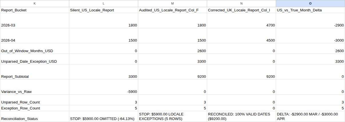
Put the reconciliation block in Raw_Export!K1:O10. Format K2:K3 as Plain text in Google Sheets or Text in Excel before entering 2026-03 and 2026-04:
| Row | Report_Bucket (K) | Silent_US_Locale_Report (L) | Audited_US_Locale_Report_Col_F (M) | Corrected_UK_Locale_Report_Col_I (N) | US_vs_True_Month_Delta (O) |
|---|---|---|---|---|---|
| 2 | 2026-03 | $1,800.00 | $1,800.00 | $4,700.00 | -$2,900.00 |
| 3 | 2026-04 | $1,500.00 | $1,500.00 | $4,500.00 | -$3,000.00 |
| 4 | Out_of_Window_Months_USD | $0.00 | $2,600.00 | $0.00 | +$2,600.00 |
| 5 | Unparsed_Date_Exception_USD | $0.00 | $3,300.00 | $0.00 | +$3,300.00 |
| 6 | Report_Subtotal | $3,300.00 | $9,200.00 | $9,200.00 | $0.00 |
| 7 | Variance_vs_Raw | -$5,900.00 | $0.00 | $0.00 | $0.00 |
| 8 | Unparsed_Row_Count | 3 | 3 | 0 | 3 |
| 9 | Exception_Row_Count | 5 | 5 | 0 | 5 |
| 10 | Reconciliation_Status | STOP: $5900.00 OMITTED (-64.13%) | STOP: $5900.00 LOCALE EXCEPTIONS (5 ROWS) | RECONCILED: 100% VALID DATES ($9200.00) | DELTA: -$2900.00 MAR / -$3000.00 APR |
- Silent US-locale report (
Col L): Sums March ($1,800.00) and April ($1,500.00) fromCol F, reporting $3,300.00 and omitting $5,900.00 (-64.13%). - Audited US-locale report (
Col M): Adds $2,600.00 inM4and $3,300.00 inM5. Its subtotal (M6) reaches $9,200.00 ($0.00 variance inM7), butM8(3 unparsed rows) andM9(5 exception rows) triggerSTOP: $5900.00 LOCALE EXCEPTIONS (5 ROWS). Even on a test copy where Row 8 has an invalid date with $0.00 (C8="31/04/2026",D8=0),N8:N9stopN10withSTOP: $0.00 LOCALE EXCEPTIONS (1 ROWS)(restore Row 8 afterward). - Corrected UK-locale report (
Col N): Reports $4,700.00 in March, $4,500.00 in April, 0 exceptions, andRECONCILED: 100% VALID DATES ($9200.00). This verifiesA2:I8holds validDD/MM/YYYYdates (2000–2099) across2026-03and2026-04; it does not check duplicate IDs, rows below row 8, or omitted invoices, so tie outCOUNTA(A2:A8)andSUM(D2:D8)against your billing system.
Copy-Paste Formula Reference
Enter in L2:M2 (copy to L3:M3), put =IF(NOT(ISNUMBER(L2)), "CHECK INPUTS", 0) in L4:L5, and enter in N2 (copy to N3):
=IF(OR(COUNTA($A$2:$A$8)<7, COUNT($D$2:$D$8)<>COUNTA($A$2:$A$8), COUNTIF($G$2:$G$8, "CHECK INPUTS")>0, COUNTIF($F$2:$F$8, "CHECK INPUTS")>0), "CHECK INPUTS", SUMIFS($D$2:$D$8, $F$2:$F$8, $K2))
=IF(OR(COUNTA($A$2:$A$8)<7, COUNT($D$2:$D$8)<>COUNTA($A$2:$A$8), COUNTIF($G$2:$G$8, "CHECK INPUTS")>0, COUNTIF($I$2:$I$8, "CHECK INPUTS")>0), "CHECK INPUTS", SUMIFS($D$2:$D$8, $I$2:$I$8, $K2))
In M4 and N4, use SUMPRODUCT (in Google Sheets en_US, "<>"&$K$2 in SUMIFS coerces "2026-03" to a date serial):
=IF(NOT(ISNUMBER(M2)), "CHECK INPUTS", SUMPRODUCT($D$2:$D$8, --($F$2:$F$8<>$K$2), --($F$2:$F$8<>$K$3), --($F$2:$F$8<>"UNPARSED TEXT DATE"), --($F$2:$F$8<>"DATE PARSE EXCEPTION")))
=IF(NOT(ISNUMBER(N2)), "CHECK INPUTS", SUMPRODUCT($D$2:$D$8, --($I$2:$I$8<>$K$2), --($I$2:$I$8<>$K$3), --($I$2:$I$8<>"UNPARSED TEXT DATE"), --($I$2:$I$8<>"DATE PARSE EXCEPTION")))
In M5 and N5, then L6 (copy to M6:N6) and L7 (copy to M7:N7):
=IF(NOT(ISNUMBER(M2)), "CHECK INPUTS", SUMIFS($D$2:$D$8, $F$2:$F$8, "UNPARSED TEXT DATE") + SUMIFS($D$2:$D$8, $F$2:$F$8, "DATE PARSE EXCEPTION"))
=IF(NOT(ISNUMBER(N2)), "CHECK INPUTS", SUMIFS($D$2:$D$8, $I$2:$I$8, "UNPARSED TEXT DATE") + SUMIFS($D$2:$D$8, $I$2:$I$8, "DATE PARSE EXCEPTION"))
=IF(COUNT(L2:L5)<4, "CHECK INPUTS", SUM(L2:L5))
=IF(NOT(ISNUMBER(L6)), "CHECK INPUTS", ROUND(L6 - SUM($D$2:$D$8), 2))
In L8 (use M7 in M8), N8, L9 (use M8 in M9), and N9:
=IF(NOT(ISNUMBER(L7)), "CHECK INPUTS", COUNTIF($F$2:$F$8, "UNPARSED TEXT DATE") + COUNTIF($F$2:$F$8, "DATE PARSE EXCEPTION"))
=IF(NOT(ISNUMBER(N7)), "CHECK INPUTS", COUNTIF($I$2:$I$8, "UNPARSED TEXT DATE") + COUNTIF($I$2:$I$8, "DATE PARSE EXCEPTION"))
=IF(NOT(ISNUMBER(L8)), "CHECK INPUTS", COUNTA($A$2:$A$8) - (COUNTIF($F$2:$F$8, $K$2) + COUNTIF($F$2:$F$8, $K$3)))
=IF(NOT(ISNUMBER(N8)), "CHECK INPUTS", COUNTA($A$2:$A$8) - (COUNTIF($I$2:$I$8, $K$2) + COUNTIF($I$2:$I$8, $K$3)))
In L10, M10, and N10:
=IF(NOT(ISNUMBER(L9)), "CHECK INPUTS", IF(L7<>0, "STOP: $" & TEXT(ABS(L7), "0.00") & " OMITTED (" & TEXT(L7/SUM($D$2:$D$8), "0.00%") & ")", IF(OR(ROUND(L4+L5, 2)>0, L8>0, L9>0), "STOP: $" & TEXT(L4+L5, "0.00") & " LOCALE EXCEPTIONS (" & L9 & " ROWS)", "RECONCILED: 100% VALID DATES ($" & TEXT(L6, "0.00") & ")")))
=IF(NOT(ISNUMBER(M9)), "CHECK INPUTS", IF(M7<>0, "STOP: $" & TEXT(ABS(M7), "0.00") & " OMITTED (" & TEXT(M7/SUM($D$2:$D$8), "0.00%") & ")", IF(OR(ROUND(M4+M5, 2)>0, M8>0, M9>0), "STOP: $" & TEXT(M4+M5, "0.00") & " LOCALE EXCEPTIONS (" & M9 & " ROWS)", "RECONCILED: 100% VALID DATES ($" & TEXT(M6, "0.00") & ")")))
=IF(NOT(ISNUMBER(N9)), "CHECK INPUTS", IF(N7<>0, "STOP: $" & TEXT(ABS(N7), "0.00") & " OMITTED (" & TEXT(N7/SUM($D$2:$D$8), "0.00%") & ")", IF(OR(ROUND(N4+N5, 2)>0, N8>0, N9>0), "STOP: $" & TEXT(N4+N5, "0.00") & " LOCALE EXCEPTIONS (" & N9 & " ROWS)", "RECONCILED: 100% VALID DATES ($" & TEXT(N6, "0.00") & ")")))
Enter the first delta formula in O2 and fill through O7; enter the next in O8 and fill to O9; and enter the status formula in O10:
=IF(OR(NOT(ISNUMBER(M2)), NOT(ISNUMBER(N2))), "CHECK INPUTS", ROUND(M2 - N2, 2))
=IF(OR(NOT(ISNUMBER(M8)), NOT(ISNUMBER(N8))), "CHECK INPUTS", M8 - N8)
=IF(OR(M10="CHECK INPUTS", N10="CHECK INPUTS"), "CHECK INPUTS", "DELTA: " & IF(O2<0, "-$"&TEXT(ABS(O2),"0.00"), "+$"&TEXT(O2,"0.00")) & " MAR / " & IF(O3<0, "-$"&TEXT(ABS(O3),"0.00"), "+$"&TEXT(O3,"0.00")) & " APR")
Frequently Asked Questions
Should I change File > Settings > Locale to United Kingdom in Google Sheets?
Only if the whole workbook uses UK dates, currency, and regional rules. In a US-locale workbook, keep United States, import Col C as text, convert D2:D8 with =VALUE(TRIM(D2)) pasted as values, and build numeric DATE serials in Col H.
How do I keep the date interpretation consistent across machines?
A plain Change Type > Date step without a locale argument evaluates dates using the effective query or workbook locale. Passing "en-GB" via Change Type > Using Locale… locks the culture parameter in the M step across machines.
What to Do Next
Once N10 reads RECONCILED: 100% VALID DATES ($9200.00), use Col H or Col I to build a monthly sales pivot table in Google Sheets or update your monthly KPI scorecard. Before sending the report out, run through the small business data audit checklist.