
To standardize customer names in a spreadsheet, build a mapping table, sometimes called a crosswalk. Each row pairs one spelling from your export with one customer ID and one approved name. Then look up each invoice’s cleaned name with an exact-match XLOOKUP that returns “UNMAPPED NAME” when a spelling is missing. Skip approximate lookups and unreviewed fuzzy matches, and check the mapped totals against the export.
In the April example below, 8 invoices use 7 different spellings for 4 real customers. Grouped by the raw names, Summit Precision Tool looks like the top customer at $1,800.00. Mapped to IDs, Beacon Dental Clinic is the top customer, billed under three different names: $1,400.00 + $1,600.00 + $900.00 = $3,900.00.
My preferred tool is Google Sheets because a spreadsheet should be shareable. It should make collaborating with others easy. Every step below also covers Excel for the web. If your export already has a customer ID column, you’re one step further along, so find unmatched customer IDs with XLOOKUP instead. To keep new entries consistent from now on, use dropdowns to keep spreadsheet categories consistent. This article fixes the names that are already in your exports.
Unless a step says otherwise, the results below come from a test of this exact workbook in Google Sheets and Excel for the web, both in US English. Desktop Excel, Excel 2016 and 2019, and Power Query weren’t part of the test.
The Example Export
Below is the 8-row invoice export I made up for this article. It sits on a sheet named Customer_Map, with headings in A1:D1 and invoices in rows 2 to 9. The Row column is a row-number guide, not a worksheet column.
| Row | invoice_id (A) | invoice_date (B) | customer_name_raw (C) | net_sales_usd (D) |
|---|---|---|---|---|
| 2 | INV-7101 | 2026-04-03 | Beacon Dental Clinic | $1,400.00 |
| 3 | INV-7102 | 2026-04-06 | Beacon Dental Lab | $1,500.00 |
| 4 | INV-7103 | 2026-04-09 | Redwood Cold Storage | $1,700.00 |
| 5 | INV-7104 | 2026-04-12 | Beacon Dental Clinic, LLC | $1,600.00 |
| 6 | INV-7105 | 2026-04-15 | Summit Precision Tool | $1,000.00 |
| 7 | INV-7106 | 2026-04-19 | Redwood Cold Storage Co. | $1,100.00 |
| 8 | INV-7107 | 2026-04-23 | BDC – Downtown | $900.00 |
| 9 | INV-7108 | 2026-04-28 | Summit Precision Tool | $800.00 |
The export totals $10,000.00. It has no customer ID, only the name someone typed on each invoice. Rows 2, 5, and 8 are the same dental clinic. Row 3 is a different business, a dental lab, that happens to share the first two words. Rows 4 and 7 are the same cold-storage company.
Here are five ways of grouping this export report. The last two rows assume next month’s export spells row 8 as Beacon Dental Office, a spelling the crosswalk doesn’t have yet.
| Method | Invoices | Total sales | Customers | Top customer |
|---|---|---|---|---|
Crosswalk with exact XLOOKUP |
8 | $10,000.00 | 4 | $3,900.00 |
| Group on the raw names | 8 | $10,000.00 | 7 | $1,800.00 |
| Fuzzy or prefix match merges Clinic and Lab (hypothetical) | 8 | $10,000.00 | 3 | $5,400.00 |
| Approximate lookup on the new spelling | 8 | $10,000.00 | 4 | $3,000.00 |
| Exact lookup with a blank error fallback | 7 | $9,100.00 | 4 | $3,000.00 |
Only the first row is right. Three of the wrong ones still total $10,000.00, so a total check alone won’t catch them.
Why Common Shortcuts Misassign Customers
Grouping on raw names. A pivot table or SUMIFS on column C treats every spelling as its own customer. Seven groups come back instead of four. Beacon Dental Clinic’s $3,900.00 splits into $1,400.00, $1,600.00, and $900.00, so Summit Precision Tool looks like the biggest customer at $1,800.00. Any repeat-customer rate or customer concentration check built on those groups is wrong, too.
Find and Replace on the export. Replacing “Beacon Dental Clinic, LLC” with “Beacon Dental Clinic” in column C fixes this month. It leaves no record of what changed, and next month’s export brings the old spelling back. A crosswalk keeps each decision in one row you can review.
To try the next two shortcuts yourself, build the workbook in Step 1 and Step 2 first. Then duplicate the Customer_Map tab and run the experiments on the copy, so the original stays as your unchanged benchmark. On the copy, change C8 to Beacon Dental Office, as if next month’s export spelled it that way, and type each test formula in an empty cell outside the tables, such as Y8.
Approximate lookup. VLOOKUP with its fourth argument left out or set to TRUE assumes a sorted list and returns the closest smaller match. On the A–Z crosswalk below, that’s Beacon Dental Lab, so VLOOKUP(F8, $K$2:$L$8, 2, TRUE) returns the lab’s ID, CUST-102. XLOOKUP(F8, $K$2:$K$8, $L$2:$L$8, "UNMAPPED NAME", -1). With match mode -1, it did the same. In a report that fills either lookup down all eight invoices, the $900.00 goes to the lab. Beacon Dental Lab rises from $1,500.00 to $2,400.00, Beacon Dental Clinic drops from $3,900.00 to $3,000.00, and the total still reads $10,000.00. Nothing on the sheet looks like an error.
Sorting doesn’t make approximate matching safe. With the crosswalk sorted Z–A, the approximate VLOOKUP returned the clinic’s ID for Beacon Dental Office. It also returned the clinic’s ID for Summit Precision Tool, a name that’s in the list exactly. Both programs gave the same results. On an unsorted list, an approximate VLOOKUP can misroute even a correct spelling. XLOOKUP with match mode -1 returned the lab’s ID whether the list was sorted A–Z or Z–A, because its default search runs from top to bottom and doesn’t need a sorted list.
A blank error fallback. On the same copy, an exact lookup with no fallback, such as XLOOKUP(F8, $K$2:$K$8, $L$2:$L$8) or VLOOKUP(F8, $K$2:$L$8, 2, FALSE), returns #N/A for Beacon Dental Office. That error is useful because you can see it. Wrapping the lookup as IFERROR(XLOOKUP(F8, $K$2:$K$8, $L$2:$L$8), "") hides it, and the cell goes blank. In a report that fills the wrapped lookup down all eight invoices, SUMIFS skips the blank row, and the report shows 7 invoices and $9,100.00 with no warning. The fix is a fallback that says something. The lookup in Step 2 returns “UNMAPPED NAME” instead of a blank.
Delete the copy when you’re done. Your original Customer_Map still has BDC – Downtown in C8.
Fuzzy matching. Power Query in Excel offers a fuzzy merge for matching similar text. Microsoft documents that it scores similarity with the Jaccard method, uses a default similarity threshold of 0.80, ignores case by default, and returns every match above the threshold unless you set a maximum number of matches. Set it to 1 to keep one match per row. Power Query wasn’t run for this article, so the numbers that follow are hypothetical. If a fuzzy match or a “starts with Beacon Dental” rule merged Beacon Dental Lab into Beacon Dental Clinic, you’d get 3 customers and a top customer of $5,400.00. Two separate businesses would become one.
A lookup table that lists the same alias twice causes a related problem. A merge can return two rows for one invoice. In the example, a duplicated Beacon Dental Clinic alias turns 8 invoices into 9 and $10,000.00 into $11,400.00, the same fan-out that explains why merging tables inflates your sales total.
A reviewed crosswalk avoids all five problems. A person approves each spelling once, the lookup accepts only exact spellings, and any new spelling stops the report until someone adds it.
Step 1: Build the Crosswalk
The workbook uses one sheet, Customer_Map, with four blocks side by side:
A1:I9holds the invoices in columns A to D, plus helper formulas in E to I.K1:N8holds the crosswalk, with a check formula in column N.P1:S6holds the customer summary.U1:W16holds the reconciliation check.
Leave columns J, O, and T empty as spacers. Enter dates as real dates and amounts as plain numbers (1400, not “$1,400”). Then paste the formulas from the Formula Reference at the end before you try any of the experiments below.
The crosswalk has three typed columns and one check column:
| Row | alias_name (K) | customer_id (L) | canonical_name (M) | Alias_Check (N) |
|---|---|---|---|---|
| 2 | BDC – Downtown | CUST-101 | Beacon Dental Clinic | OK |
| 3 | Beacon Dental Clinic | CUST-101 | Beacon Dental Clinic | OK |
| 4 | Beacon Dental Clinic, LLC | CUST-101 | Beacon Dental Clinic | OK |
| 5 | Beacon Dental Lab | CUST-102 | Beacon Dental Lab | OK |
| 6 | Redwood Cold Storage | CUST-103 | Redwood Cold Storage | OK |
| 7 | Redwood Cold Storage Co. | CUST-103 | Redwood Cold Storage | OK |
| 8 | Summit Precision Tool | CUST-104 | Summit Precision Tool | OK |
Three rules keep it trustworthy:
- Each alias appears once. The check ignores case, so “beacon dental clinic” and “Beacon Dental Clinic” count as the same alias.
- Each customer ID has one canonical name, and each canonical name belongs to one ID.
- Each canonical name also appears as its own alias, as Beacon Dental Clinic does in row 3.
The formula in N2, copied down to N8, enforces them. It returns "OK" or one of four flags: "DUPLICATE ALIAS", "SPLIT CANONICAL" for an ID with two names, "MISSING SELF ALIAS", or "CHECK ALIAS" for a blank or badly formatted entry. Any flag stops the whole report.
The list is sorted A–Z here only so the approximate-lookup demonstration works. The exact lookup doesn’t need any order, so you can add new aliases at the bottom.
The helper formulas are strict on purpose, so the example flags a doubtful row instead of guessing. Column E marks an invoice row "CHECK ROW", and the report stops, unless all of these are true:
- The invoice ID is uppercase text with no spaces, such as INV-7101, and appears only once. The duplicate check ignores case.
- The date is a whole date from 2000-01-01 to 2100-01-01, with no time attached.
- The amount is a number of zero or more, with no more than two decimal places.
- Neither the invoice ID nor the customer name contains a line break or any of these characters: * ? ~ = < >
Column N applies similar rules to the crosswalk. Its text must already be trimmed, and every customer ID must be CUST- followed by three digits, such as CUST-101. The summary IDs in column P follow the same format. These are rules of this example workbook, not limits of XLOOKUP. A credit memo of -250, a date with a time, or an ID like C-104 fails the check. If your export has credits or a different ID format, redesign and retest the checks before you rely on them.
Raw names in column C don’t need to be tidy. Extra spaces and non-breaking spaces are fine there, because column F cleans them before the lookup. Column E checks the row but doesn’t change it.
If other people edit the workbook, protect the formula cells and the crosswalk in columns K to N, so only the person who approves aliases can change them.
Step 2: Look Up Each Invoice’s Customer ID
Column F cleans the raw name:
=IF(NOT(EXACT(E2, "OK")), "", TRIM(SUBSTITUTE(C2, CHAR(160), " ")))
SUBSTITUTE turns non-breaking spaces, which often come from web exports, into normal spaces. TRIM then removes spaces at the start and end and shrinks repeated spaces to one. Microsoft notes that TRIM alone doesn’t remove non-breaking spaces, which is why the formula needs both.
The lookup itself is one XLOOKUP with five arguments:
=XLOOKUP(F2, $K$2:$K$8, $L$2:$L$8, "UNMAPPED NAME", 0)
It looks for the cleaned name in the alias column and returns the customer ID from column L. The fourth argument is the text to show when the name isn’t in the list. The fifth, 0, asks for an exact match. That’s also the default, but writing it makes the intent clear to the next person who opens the sheet.
The full G2 in the Formula Reference wraps this lookup in checks, so it returns "CHECK INPUTS" if any invoice row or crosswalk row fails. H2 returns the canonical name from column M the same way. It also confirms that the customer ID exists in the summary in P2:P5, and returns "UNLISTED SUMMARY ID" if it doesn’t. I2 marks the first row of each distinct cleaned name with 1, so SUM(I2:I9) counts the 7 raw spellings. Enter E2:I2 and copy them down to row 9.
| Row | customer_name_raw (C) | Mapped_Customer_ID (G) | Mapped_Customer_Name (H) |
|---|---|---|---|
| 2 | Beacon Dental Clinic | CUST-101 | Beacon Dental Clinic |
| 3 | Beacon Dental Lab | CUST-102 | Beacon Dental Lab |
| 4 | Redwood Cold Storage | CUST-103 | Redwood Cold Storage |
| 5 | Beacon Dental Clinic, LLC | CUST-101 | Beacon Dental Clinic |
| 6 | Summit Precision Tool | CUST-104 | Summit Precision Tool |
| 7 | Redwood Cold Storage Co. | CUST-103 | Redwood Cold Storage |
| 8 | BDC – Downtown | CUST-101 | Beacon Dental Clinic |
| 9 | Summit Precision Tool | CUST-104 | Summit Precision Tool |

The match ignores case. In the test, C2 was changed to “beacon dental clinic” in lowercase, with extra spaces in front, between the words, and at the end, including two non-breaking spaces. Column E still said OK, column F returned “beacon dental clinic”, and G2 still returned CUST-101 in both programs.
The summary in P1:S6 lists each customer once. Type the IDs and canonical names in P2:Q5. R2 counts the customer’s invoices with COUNTIF, and S2 adds their sales with SUMIFS on the mapped ID in column G. Copy both down to row 5. Row 6 holds the totals, labeled Mapped_Summary_Total in P6 and ALL_MAPPED in Q6.
| Row | customer_id (P) | canonical_name (Q) | invoice_count (R) | net_sales_usd (S) |
|---|---|---|---|---|
| 2 | CUST-101 | Beacon Dental Clinic | 3 | $3,900.00 |
| 3 | CUST-102 | Beacon Dental Lab | 1 | $1,500.00 |
| 4 | CUST-103 | Redwood Cold Storage | 2 | $2,800.00 |
| 5 | CUST-104 | Summit Precision Tool | 2 | $1,800.00 |
| 6 | Mapped_Summary_Total | ALL_MAPPED | 8 | $10,000.00 |

Beacon Dental Clinic is now the top customer at $3,900.00, and Summit Precision Tool drops to third.
XLOOKUP isn’t available in Excel 2016 or Excel 2019. For those versions, the Formula Reference includes replacement G2 and H2 formulas that use INDEX, MATCH with a match type of 0, and IFNA. Replace both, so no XLOOKUP is left on the sheet. In the test, the replacements gave the same results as the XLOOKUP versions in Google Sheets and Excel for the web, including the stops for a missing alias and a missing summary ID. Excel 2016 and 2019 themselves weren’t tested.
To see what a new spelling does, duplicate the Customer_Map tab again and work on the copy. Change C8 on the copy to Beacon Dental Office, as if next month’s export used a new spelling. G8 and H8 show “UNMAPPED NAME”. The summary total in S6 drops to $9,100.00, and the status in V16 says STOP: CROSSWALK OMITS $900.00 (1 UNMAPPED CUSTOMER ROW). That’s the result you want: the report stops until a person confirms who Beacon Dental Office is.
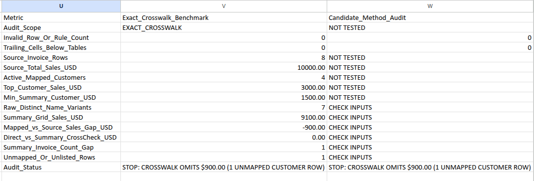
If it’s the clinic, the fix is one new crosswalk row. On the copy, add Beacon Dental Office, CUST-101, Beacon Dental Clinic in K9:M9. Until you resize the crosswalk ranges, V16 says STOP: TRAILING CROSSWALK ROWS OUTSIDE LOOKUP RANGE (RESIZE CROSSWALK), because row 9 sits below the lookup range. After the resize described in the section on export size below, G8 should return CUST-101 and V16 should reconcile at $10,000.00 again. The test didn’t run this exact repair, but it grew the crosswalk the same way with other new aliases, and both programs reconciled.
Delete the copy before Step 3. The original Customer_Map should still have BDC – Downtown in C8, seven aliases ending in row 8, four customers in the summary, and NOT TESTED in W2.
Step 3: Reconcile the Mapped Totals
The check block in U1:W16 answers two questions. Column V asks whether the crosswalk and summary account for every invoice in the export. Column W lets you test another report against that benchmark, such as a pivot table or a dashboard someone else built.
| Row | Metric (U) | Column V at baseline | What goes in column W |
|---|---|---|---|
| 2 | Audit_Scope | EXACT_CROSSWALK (typed) | Type NOT TESTED, or EXACT_CROSSWALK when you enter readings |
| 3 | Invalid_Row_Or_Rule_Count | 0 | Type 0 |
| 4 | Trailing_Cells_Below_Tables | 0 | Type 0 |
| 5 | Source_Invoice_Rows | 8 | Invoice count from the other report |
| 6 | Source_Total_Sales_USD | 10000.00 | Total sales from the other report |
| 7 | Active_Mapped_Customers | 4 | Number of customers with at least one invoice in the other report |
| 8 | Top_Customer_Sales_USD | 3900.00 | Largest customer total in the other report |
| 9 | Min_Summary_Customer_USD | 1500.00 | Smallest customer total in the other report |
| 10 | Raw_Distinct_Name_Variants | 7 | Formula: other report’s customers minus the summary’s |
| 11 | Summary_Grid_Sales_USD | 10000.00 | Formula: other report’s sales minus the summary’s |
| 12 | Mapped_vs_Source_Sales_Gap_USD | 0.00 | Formula: other report’s sales minus the source’s |
| 13 | Direct_vs_Summary_CrossCheck_USD | 0.00 | Formula: shift in the top and smallest customer totals |
| 14 | Summary_Invoice_Count_Gap | 0 | Formula: other report’s invoices minus the source’s |
| 15 | Unmapped_Or_Unlisted_Rows | 0 | Formula: input checks, then the invoice count gap |
| 16 | Audit_Status | Status message | Status message |
V3 counts invalid or blank cells across all three tables. V4 is the guard for rows added below a table. It counts every filled cell in columns A to I, K to N, and P to S, and subtracts the cells inside each table. Anything below the tables, whether in row 10 or row 500, makes it greater than 0 and stops the report. V15 counts invoices marked “UNMAPPED NAME” or “UNLISTED SUMMARY ID”.
V7 counts only customers with at least one invoice, so enter the same count in W7 and leave out customers with no invoices this month. V9 works the other way. It’s the smallest total across every summary row, including a customer at $0.00. Read W9 the same way, and include customers that show $0.00 in the other report.
Until you have readings, leave W2 and W5:W9 at NOT TESTED and W3:W4 at 0. To check a report, type EXACT_CROSSWALK in W2 and the five readings in W5:W9. Set them back to NOT TESTED after each check, so one test doesn’t carry into the next.
Here’s what W16 said for each shortcut from earlier:
| Report being checked | Readings in W5:W9 | W16 says |
|---|---|---|
| Matches the crosswalk | 8, 10000, 4, 3900, 1500 | RECONCILED: CANDIDATE TOTALS AND BOUNDS MATCH CROSSWALK ($10000.00 ACROSS 4 CUSTOMERS) |
| Grouped on raw names | 8, 10000, 7, 1800, 900 | STOP: CUSTOMER COUNT MISMATCH (7 VS 4; UNMAPPED NAME VARIANTS SPLIT ACCOUNTS) |
| Clinic and Lab merged (hypothetical) | 8, 10000, 3, 5400, 1800 | STOP: FALSE ENTITY MERGE (3 VS 4 CUSTOMERS; DISTINCT ACCOUNTS COLLAPSED) |
| Approximate lookup on Beacon Dental Office | 8, 10000, 4, 3000, 1800 | STOP: CUSTOMER TOTALS MISROUTED ($1200.00 TOP/MIN SHIFT; CHECK APPROXIMATE OR WRONG ALIAS) |
| Blank error fallback | 7, 9100, 4, 3000, 1500 | STOP: CANDIDATE INVOICE COUNT MISMATCH (7 VS 8; $900.00 SALES GAP) |
| Duplicated alias | 9, 11400, 4, 5300, 1500 | STOP: CANDIDATE INVOICE COUNT MISMATCH (9 VS 8; $1400.00 SALES GAP) |
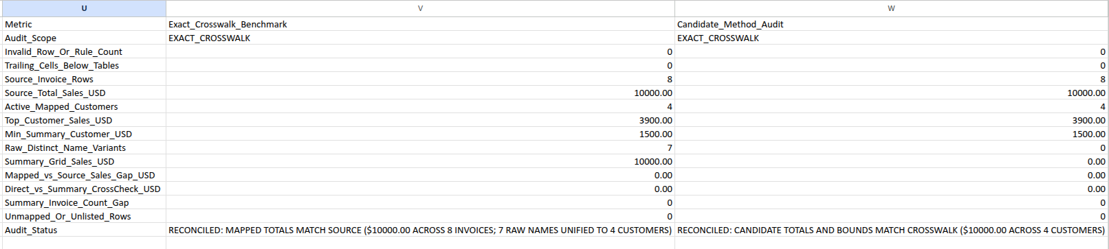
In the test, the raw-name, approximate-lookup, and blank-fallback readings came from small probe reports built on separate sheets in both programs. The merge and duplicated-alias readings were typed in to match those mistakes, because Power Query wasn’t run.
The approximate lookup is the case a total check misses. The invoice count, total, and customer count all match. Only the bounds move: the top customer falls by $900.00 and the smallest rises by $300.00, so W13 shows 1200.00 and the report stops.
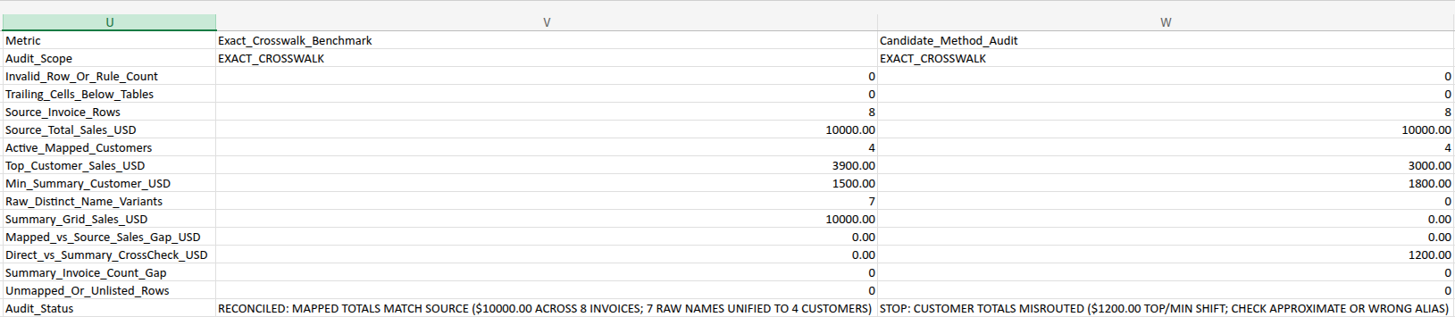
Column V also stops on its own when the workbook itself changes. These are the live edits from the test. To repeat one, start from a fresh duplicate of the untouched Customer_Map tab, make that single change on the copy, and delete the copy afterward:
| Change on Customer_Map | V16 says |
|---|---|
C8 = Beacon Dental Office |
STOP: CROSSWALK OMITS $900.00 (1 UNMAPPED CUSTOMER ROW) |
K4 = beacon dental clinic |
STOP: DUPLICATE ALIAS IN CROSSWALK (EACH ALIAS MUST BE UNIQUE) |
| New alias in row 9, ranges not resized | STOP: TRAILING CROSSWALK ROWS OUTSIDE LOOKUP RANGE (RESIZE CROSSWALK) |
Changing W2:W9 back to NOT TESTED and 0 doesn’t undo an edit like these, so use a new copy for each one. When column V stops, column W shows the same message, so fix the workbook before you check any other report.
When Next Month’s Export Changes Size
Each table can grow or shrink on its own. Every range in the formulas ends at a fixed last row, so a resize means replacing the old last row with the new one inside the formulas.
Find the last rows before you change anything:
- Invoices: the invoice count plus 1. Eight invoices end at row 9.
- Crosswalk: the alias count plus 1. Seven aliases end at row 8.
- Summary: the customer count plus 1 for the last customer, and plus 2 for the totals row. Four customers end at row 5, with totals in row 6.
Then choose the Find and Replace option. Select from E2 across to column W, down to the largest of these: row 16, the invoice last row, the crosswalk last row, and the summary totals row. In the example, that’s E2:W16. With 23 aliases and 20 customers, the crosswalk ends at row 24, so you’d select E2:W24.
The selection has to reach every summary row because the summary formulas also read the invoice ranges. In the test, a workbook with 8 invoices, 23 aliases, and 20 customers added a ninth invoice for $1,100.00 using only E2:W16. One customer’s summary formulas kept the old invoice range, and V16 said STOP: SUMMARY DIFFERS FROM SOURCE BY $1100.00. With E2:W24, it reconciled at $11,100.00 across 9 invoices.
To resize the invoices:
- When the export grows, type the new invoices in columns A to D below the old last row, and leave E to I empty in those rows for now. When it shrinks, don’t clear anything yet.
- In your selection, replace
:$A$followed by the old last row with:$A$followed by the new last row. Do the same for columns B to I, so nine replacements in all. Going from 8 invoices to 9, that’s:$A$9to:$A$10, through:$I$9to:$I$10. - When the export grows, copy
E2:I2down to the new last row. When it shrinks, clear the unused cells in A to I only, from the row below the new last row down to the old last row.
To resize the crosswalk, follow the same steps on columns K to M. Replace the old last row in :$K$, :$L$, :$M$, and :$N$, so four replacements. Then copy N2 down to the new last row, or clear the unused cells in K to N. Adding Beacon Dental Office as an eighth alias means replacing :$K$8 with :$K$9, and the same for L, M, and N.
To resize the summary, move the totals row with Insert cells, so the other tables stay where they are.
- Growing from 4 customers to 5: Select
P6:S6and insert cells, shifting down. In Google Sheets, that’s Insert > Cells > Insert cells and shift down. In Excel for the web, it’s Home > Insert > Insert Cells & Shift Down. The totals move to row 7, and both programs updated the formulas automatically, which point at the totals row on their own. Type the new ID and name inP6:Q6. Then select fromE2across to column W, down to the largest of row 16, the invoice last row, the crosswalk last row, and the new totals row. In the example, that’s stillE2:W16. Replace:$P$5with:$P$6, and the same for Q, R, and S. Then copyR2:S2down to row 6. - Shrinking: Make the four replacements first, using the same full selection, with the current totals row as the last term. Then select the unused summary rows in P to S and delete cells, shifting up. In Google Sheets, that’s Edit > Delete > Cells and shift up. In Excel for the web, it’s Home > Delete > Delete Cells & Shift Up.
For the replacements, keep Find and Replace inside your selection and make it search the formulas:
- Google Sheets: Choose Edit > Find and replace, set Search to Specific range, and check Also search within formulas. Leave Match entire cell contents unchecked. In the test, the formulas checkbox was unchecked every time the dialog opened, so check it each time. Leave Search using regular expressions unchecked too, because the $ sign has a special meaning there.
- Excel for the web: Choose Home > Find & Select > Replace, set Within to Selection under the search options, and leave Match entire cell contents unchecked. The tested dialog had no option for searching formulas, and Replace All changed the formula references in the selection directly.
Replace only those strings, and always start from the current last row. Never insert or delete whole worksheet rows, because that moves or cuts the tables beside the one you’re changing. The test shrank the invoices from 8 to 4 and grew them to 9, while the crosswalk went from 7 to 4 to 8. It also ran an export of 105 invoices and added a fifth customer, Cedar Ridge Logistics, across all three tables. Every chain reconciled in both programs.
What These Checks Can’t Prove
The check in column W compares five numbers. It doesn’t compare each customer. If another report moves $100.00 from Redwood Cold Storage to Summit Precision Tool, showing $2,700.00 and $1,900.00, the count, total, customer count, top, and smallest totals all stay the same. In the test, W16 still said reconciled. Compare each customer’s ID, invoice count, and total in the other report against P2:S5 before you trust the split by customer.
A crosswalk can also be consistent and still wrong. If BDC – Downtown were mapped to CUST-102 by mistake, every check would pass, and V16 would reconcile at $10,000.00. Only a person can confirm who an alias belongs to. For any doubtful spelling, check the billing address, tax ID, or contract before you add it.
The check also can’t tell you whether an invoice was missing from the export. Compare the invoice count in V5 and the total in V6 with your billing or point-of-sale system for the same dates.
Frequently Asked Questions
Should customer name mapping be case-sensitive?
Usually not. An exact-match XLOOKUP ignores case, so “beacon dental clinic” finds Beacon Dental Clinic. The duplicate check in column N ignores case too, so the crosswalk can’t hold two capitalizations of one name with different IDs. Customer IDs are different. The checks compare them with EXACT, so CUST-101 has to be uppercase.
Can I use INDEX and MATCH in Excel 2016 or 2019?
Yes. Replace both G2 and H2 with the replacement formulas in the Formula Reference, and copy them down to row 9. MATCH with a match type of 0 is an exact match, but it treats * and ? as wildcards, and ~ is the character that cancels them. This workbook blocks all three characters in columns E and N, so keep those checks in place. The replacements were tested in Google Sheets and Excel for the web, not in Excel 2016 or 2019.
What if two different companies have the same billing name?
A name-only crosswalk can’t separate them, because each alias maps to one ID. You’d need a combined key built from the name and something that tells the companies apart, such as the billing ZIP code or an account number, in both the invoices and the crosswalk. Use a separator the checks allow, such as |. That’s a separate workbook design, not a small edit to this one. The cleaning formula, the lookup, and every duplicate and self-alias check need to be rebuilt and retested. Keep ZIP codes as text, so you don’t lose leading zeros when you import the CSV.
What to Do Next
Once every invoice carries a stable ID, use column G instead of the raw names for any customer metric, such as repeat-customer rate or revenue concentration. When a new spelling shows up, confirm who it is, add one crosswalk row, resize the crosswalk, and check that V16 reconciles before you share the report. If you clean the export in other ways first, make the crosswalk one step in a repeatable workflow for cleaning business spreadsheet data.
Formula Reference
Each label before = names the destination cell; paste only the formula. Fill E2:I2 down to row 9 and N2 down to N8. Fill R2:S2 down to row 5. Paste R6, S6, and the column V and W formulas one cell at a time.
Headings: A1:I1 are invoice_id, invoice_date, customer_name_raw, net_sales_usd, Row_Check, Normalized_Name, Mapped_Customer_ID, Mapped_Customer_Name, and First_Raw_Name_Flag. K1:N1 are alias_name, customer_id, canonical_name, and Alias_Check. P1:S1 are customer_id, canonical_name, invoice_count, and net_sales_usd. U1:W1 are Metric, Exact_Crosswalk_Benchmark, and Candidate_Method_Audit, with the metric labels from the check-block table in U2:U16.
Typed inputs: P6 = Mapped_Summary_Total, Q6 = ALL_MAPPED, V2 = EXACT_CROSSWALK, W2 = NOT TESTED, W3 and W4 = 0, and W5:W9 = NOT TESTED.
Invoice helpers:
E2: =IF(OR(COUNTA(A2:D2)<4, NOT(ISTEXT(A2)), NOT(ISNUMBER(B2)), NOT(ISTEXT(C2)), NOT(ISNUMBER(D2)), TRIM(SUBSTITUTE(A2, CHAR(160), " "))="", TRIM(SUBSTITUTE(C2, CHAR(160), " "))="", NOT(EXACT(A2, TRIM(SUBSTITUTE(A2, CHAR(160), " ")))), NOT(EXACT(A2, UPPER(A2))), NOT(ISERROR(FIND(" ", A2))), NOT(ISERROR(FIND(CHAR(10), A2&C2))), NOT(ISERROR(FIND(CHAR(13), A2&C2))), NOT(ISERROR(FIND("*", A2&C2))), NOT(ISERROR(FIND("?", A2&C2))), NOT(ISERROR(FIND("~", A2&C2))), NOT(ISERROR(FIND("=", A2&C2))), NOT(ISERROR(FIND("<", A2&C2))), NOT(ISERROR(FIND(">", A2&C2)))), "CHECK ROW", IF(OR(INT(B2)<>B2, B2<DATE(2000,1,1), B2>DATE(2100,1,1), D2<0, ROUND(D2, 2)<>D2, SUMPRODUCT(--(UPPER($A$2:$A$9)=UPPER(A2)))>1), "CHECK ROW", "OK"))
F2: =IF(NOT(EXACT(E2, "OK")), "", TRIM(SUBSTITUTE(C2, CHAR(160), " ")))
G2: =IF(OR(NOT(EXACT(E2, "OK")), COUNTIF($E$2:$E$9, "OK")<ROWS($A$2:$A$9), COUNTIF($N$2:$N$8, "OK")<ROWS($K$2:$K$8)), "CHECK INPUTS", XLOOKUP(F2, $K$2:$K$8, $L$2:$L$8, "UNMAPPED NAME", 0))
H2: =IF(EXACT(G2, "CHECK INPUTS"), "CHECK INPUTS", IF(EXACT(G2, "UNMAPPED NAME"), "UNMAPPED NAME", IF(SUMPRODUCT(--EXACT($P$2:$P$5, G2))=0, "UNLISTED SUMMARY ID", XLOOKUP(F2, $K$2:$K$8, $M$2:$M$8, "UNMAPPED NAME", 0))))
I2: =IF(OR(NOT(EXACT(E2, "OK")), COUNTIF($E$2:$E$9, "OK")<ROWS($A$2:$A$9)), "", IF(SUMPRODUCT(--(UPPER($F$2:F2)=UPPER(F2)))=1, 1, 0))
Excel 2016 and 2019 replacements for G2 and H2 (replace both):
G2: =IF(OR(NOT(EXACT(E2, "OK")), COUNTIF($E$2:$E$9, "OK")<ROWS($A$2:$A$9), COUNTIF($N$2:$N$8, "OK")<ROWS($K$2:$K$8)), "CHECK INPUTS", IFNA(INDEX($L$2:$L$8, MATCH(F2, $K$2:$K$8, 0)), "UNMAPPED NAME"))
H2: =IF(EXACT(G2, "CHECK INPUTS"), "CHECK INPUTS", IF(EXACT(G2, "UNMAPPED NAME"), "UNMAPPED NAME", IF(SUMPRODUCT(--EXACT($P$2:$P$5, G2))=0, "UNLISTED SUMMARY ID", IFNA(INDEX($M$2:$M$8, MATCH(F2, $K$2:$K$8, 0)), "UNMAPPED NAME"))))
Crosswalk check:
N2: =IF(OR(COUNTA(K2:M2)<3, NOT(ISTEXT(K2)), NOT(ISTEXT(L2)), NOT(ISTEXT(M2)), TRIM(SUBSTITUTE(K2, CHAR(160), " "))="", TRIM(SUBSTITUTE(L2, CHAR(160), " "))="", TRIM(SUBSTITUTE(M2, CHAR(160), " "))="", NOT(EXACT(K2, TRIM(SUBSTITUTE(K2, CHAR(160), " ")))), NOT(EXACT(L2, TRIM(SUBSTITUTE(L2, CHAR(160), " ")))), NOT(EXACT(M2, TRIM(SUBSTITUTE(M2, CHAR(160), " ")))), LEN(L2)<>8, NOT(EXACT(LEFT(L2, 5), "CUST-")), NOT(ISNUMBER(FIND(MID(L2, 6, 1), "0123456789"))), NOT(ISNUMBER(FIND(MID(L2, 7, 1), "0123456789"))), NOT(ISNUMBER(FIND(MID(L2, 8, 1), "0123456789"))), NOT(ISERROR(FIND(CHAR(10), K2&L2&M2))), NOT(ISERROR(FIND(CHAR(13), K2&L2&M2))), NOT(ISERROR(FIND("*", K2&L2&M2))), NOT(ISERROR(FIND("?", K2&L2&M2))), NOT(ISERROR(FIND("~", K2&L2&M2))), NOT(ISERROR(FIND("=", K2&L2&M2))), NOT(ISERROR(FIND("<", K2&L2&M2))), NOT(ISERROR(FIND(">", K2&L2&M2)))), "CHECK ALIAS", IF(SUMPRODUCT(--(UPPER($K$2:$K$8)=UPPER(K2)))>1, "DUPLICATE ALIAS", IF(OR(SUMPRODUCT(--EXACT($L$2:$L$8, L2), --NOT(EXACT($M$2:$M$8, M2)))>0, SUMPRODUCT(--(UPPER($M$2:$M$8)=UPPER(M2)), --NOT(EXACT($L$2:$L$8, L2)))>0), "SPLIT CANONICAL", IF(SUMPRODUCT(--(UPPER($K$2:$K$8)=UPPER(M2)), --EXACT($L$2:$L$8, L2))=0, "MISSING SELF ALIAS", "OK"))))
Customer summary:
R2: =IF(OR(COUNTIF($E$2:$E$9, "OK")<ROWS($A$2:$A$9), COUNTIF($N$2:$N$8, "OK")<ROWS($K$2:$K$8), COUNTIF($G$2:$G$9, "CHECK INPUTS")>0, NOT(ISTEXT($P2)), NOT(ISTEXT($Q2)), TRIM(SUBSTITUTE($P2, CHAR(160), " "))="", TRIM(SUBSTITUTE($Q2, CHAR(160), " "))="", NOT(EXACT($P2, TRIM(SUBSTITUTE($P2, CHAR(160), " ")))), NOT(EXACT($Q2, TRIM(SUBSTITUTE($Q2, CHAR(160), " ")))), LEN($P2)<>8, NOT(EXACT(LEFT($P2, 5), "CUST-")), NOT(ISNUMBER(FIND(MID($P2, 6, 1), "0123456789"))), NOT(ISNUMBER(FIND(MID($P2, 7, 1), "0123456789"))), NOT(ISNUMBER(FIND(MID($P2, 8, 1), "0123456789"))), NOT(ISERROR(FIND(CHAR(10), $P2&$Q2))), NOT(ISERROR(FIND(CHAR(13), $P2&$Q2))), NOT(ISERROR(FIND("*", $P2&$Q2))), NOT(ISERROR(FIND("?", $P2&$Q2))), NOT(ISERROR(FIND("~", $P2&$Q2))), NOT(ISERROR(FIND("=", $P2&$Q2))), NOT(ISERROR(FIND("<", $P2&$Q2))), NOT(ISERROR(FIND(">", $P2&$Q2))), SUMPRODUCT(--(UPPER($P$2:$P$5)=UPPER($P2)))>1, SUMPRODUCT(--(UPPER($Q$2:$Q$5)=UPPER($Q2)))>1, SUMPRODUCT(--EXACT($L$2:$L$8, $P2), --EXACT($M$2:$M$8, $Q2))=0), "CHECK INPUTS", COUNTIF($G$2:$G$9, $P2))
S2: =IF(NOT(ISNUMBER(R2)), "CHECK INPUTS", ROUND(SUMIFS($D$2:$D$9, $G$2:$G$9, $P2), 2))
R6: =IF(COUNT($R$2:$R$5)<ROWS($P$2:$P$5), "CHECK INPUTS", SUM($R$2:$R$5))
S6: =IF(OR(NOT(ISNUMBER($R$6)), COUNT($S$2:$S$5)<ROWS($P$2:$P$5)), "CHECK INPUTS", ROUND(SUM($S$2:$S$5), 2))
Benchmark checks:
V3: =COUNTIF($E$2:$E$9, "<>OK")+COUNTBLANK($A$2:$A$9)+COUNTBLANK($B$2:$B$9)+COUNTBLANK($C$2:$C$9)+COUNTBLANK($D$2:$D$9)+COUNTIF($N$2:$N$8, "<>OK")+COUNTBLANK($K$2:$K$8)+COUNTBLANK($L$2:$L$8)+COUNTBLANK($M$2:$M$8)+COUNTBLANK($P$2:$P$5)+COUNTBLANK($Q$2:$Q$5)
V4: =(COUNTA($A:$I)-COUNTA($A$1:$I$9))+(COUNTA($K:$N)-COUNTA($K$1:$N$8))+(COUNTA($P:$S)-COUNTA($P$1:$S$6))
V5: =IF(OR(NOT(EXACT(V2, "EXACT_CROSSWALK")), V3>0, V4>0, COUNT($I$2:$I$9)<ROWS($A$2:$A$9), NOT(ISNUMBER($R$6)), NOT(ISNUMBER($S$6))), "CHECK INPUTS", COUNTA($A$2:$A$9))
V6: =IF(NOT(ISNUMBER(V5)), "CHECK INPUTS", ROUND(SUM($D$2:$D$9), 2))
V7: =IF(NOT(ISNUMBER(V5)), "CHECK INPUTS", COUNTIF($R$2:$R$5, ">0"))
V8: =IF(NOT(ISNUMBER(V5)), "CHECK INPUTS", ROUND(MAX($S$2:$S$5), 2))
V9: =IF(NOT(ISNUMBER(V5)), "CHECK INPUTS", ROUND(MIN($S$2:$S$5), 2))
V10: =IF(NOT(ISNUMBER(V5)), "CHECK INPUTS", SUM($I$2:$I$9))
V11: =IF(NOT(ISNUMBER(V5)), "CHECK INPUTS", ROUND($S$6, 2))
V12: =IF(NOT(ISNUMBER(V5)), "CHECK INPUTS", ROUND(V11-V6, 2))
V13: =IF(NOT(ISNUMBER(V5)), "CHECK INPUTS", ROUND(ABS($S$6-SUMIFS($D$2:$D$9, $H$2:$H$9, "<>UNMAPPED NAME", $H$2:$H$9, "<>UNLISTED SUMMARY ID")), 2))
V14: =IF(NOT(ISNUMBER(V5)), "CHECK INPUTS", V5-$R$6)
V15: =IF(OR(NOT(ISNUMBER(V5)), COUNTIF($H$2:$H$9, "CHECK INPUTS")>0), "CHECK INPUTS", COUNTIF($H$2:$H$9, "UNMAPPED NAME")+COUNTIF($H$2:$H$9, "UNLISTED SUMMARY ID"))
V16: =IF(COUNTIF($E$2:$E$9, "<>OK")>0, "STOP: INVALID OR BLANK INVOICE ROWS", IF(COUNTIF($N$2:$N$8, "DUPLICATE ALIAS")>0, "STOP: DUPLICATE ALIAS IN CROSSWALK (EACH ALIAS MUST BE UNIQUE)", IF(COUNTIF($N$2:$N$8, "SPLIT CANONICAL")>0, "STOP: INCONSISTENT CANONICAL ID OR NAME IN CROSSWALK", IF(COUNTIF($N$2:$N$8, "MISSING SELF ALIAS")>0, "STOP: CANONICAL NAME MISSING SELF-ALIAS ROW IN CROSSWALK", IF(V3>0, "STOP: INVALID CROSSWALK OR SUMMARY LABELS", IF(COUNTA($K:$N)-COUNTA($K$1:$N$8)>0, "STOP: TRAILING CROSSWALK ROWS OUTSIDE LOOKUP RANGE (RESIZE CROSSWALK)", IF(COUNTA($A:$I)-COUNTA($A$1:$I$9)>0, "STOP: TRAILING INVOICE DATA OUTSIDE TABLE RANGE (RESIZE INVOICES)", IF(V4>0, "STOP: TRAILING CUSTOMER SUMMARY ROWS (RESIZE SUMMARY)", IF(NOT(ISNUMBER(V5)), "STOP: CHECK AUDIT SCOPE OR SUMMARY HEADERS", IF(AND(COUNTIF($H$2:$H$9, "UNMAPPED NAME")>0, COUNTIF($H$2:$H$9, "UNLISTED SUMMARY ID")>0), "STOP: CROSSWALK OMITS $" & TEXT(ABS(V12), "0.00") & " (" & V15 & " UNMAPPED AND UNLISTED SUMMARY ROWS)", IF(COUNTIF($H$2:$H$9, "UNMAPPED NAME")>0, "STOP: CROSSWALK OMITS $" & TEXT(ABS(V12), "0.00") & " (" & V15 & IF(V15=1, " UNMAPPED CUSTOMER ROW)", " UNMAPPED CUSTOMER ROWS)"), IF(COUNTIF($H$2:$H$9, "UNLISTED SUMMARY ID")>0, "STOP: SUMMARY OMITS $" & TEXT(ABS(V12), "0.00") & " (" & V15 & IF(V15=1, " UNLISTED CUSTOMER ID ROW)", " UNLISTED CUSTOMER ID ROWS)"), IF(OR(V12<>0, V13<>0, V14<>0, V15<>0), "STOP: SUMMARY DIFFERS FROM SOURCE BY $" & TEXT(ABS(V12), "0.00"), "RECONCILED: MAPPED TOTALS MATCH SOURCE ($" & TEXT(V6, "0.00") & " ACROSS " & V5 & " INVOICES; " & V10 & " RAW NAMES UNIFIED TO " & V7 & " CUSTOMERS)")))))))))))))
Checks for another report:
W10: =IF(EXACT(W15, "NOT TESTED"), "NOT TESTED", IF(OR(NOT(ISNUMBER(W15)), NOT(ISNUMBER(V7)), NOT(ISNUMBER(W7))), "CHECK INPUTS", W7-V7))
W11: =IF(EXACT(W15, "NOT TESTED"), "NOT TESTED", IF(OR(NOT(ISNUMBER(W15)), NOT(ISNUMBER(V11)), NOT(ISNUMBER(W6))), "CHECK INPUTS", ROUND(W6-V11, 2)))
W12: =IF(EXACT(W15, "NOT TESTED"), "NOT TESTED", IF(OR(NOT(ISNUMBER(W15)), NOT(ISNUMBER(V6)), NOT(ISNUMBER(W6))), "CHECK INPUTS", ROUND(W6-V6, 2)))
W13: =IF(EXACT(W15, "NOT TESTED"), "NOT TESTED", IF(OR(NOT(ISNUMBER(W15)), NOT(ISNUMBER(V8)), NOT(ISNUMBER(V9)), NOT(ISNUMBER(W8)), NOT(ISNUMBER(W9))), "CHECK INPUTS", ROUND(ABS(W8-V8)+ABS(W9-V9), 2)))
W14: =IF(EXACT(W15, "NOT TESTED"), "NOT TESTED", IF(OR(NOT(ISNUMBER(W15)), NOT(ISNUMBER(V5)), NOT(ISNUMBER(W5))), "CHECK INPUTS", W5-V5))
W15: =IF(OR(V3>0, V4>0, NOT(ISNUMBER(V5)), NOT(ISNUMBER(V12)), NOT(ISNUMBER(V13)), NOT(ISNUMBER(V14)), NOT(ISNUMBER(V15)), NOT(ISTEXT(W2)), NOT(ISNUMBER(W3)), NOT(ISNUMBER(W4))), "CHECK INPUTS", IF(OR(V12<>0, V13<>0, V14<>0, V15<>0, INT(W3)<>W3, W3<>0, INT(W4)<>W4, W4<>0), "CHECK INPUTS", IF(AND(EXACT(W2, "NOT TESTED"), EXACT(W5, "NOT TESTED"), EXACT(W6, "NOT TESTED"), EXACT(W7, "NOT TESTED"), EXACT(W8, "NOT TESTED"), EXACT(W9, "NOT TESTED")), "NOT TESTED", IF(OR(NOT(EXACT(W2, "EXACT_CROSSWALK")), NOT(ISNUMBER(W5)), NOT(ISNUMBER(W6)), NOT(ISNUMBER(W7)), NOT(ISNUMBER(W8)), NOT(ISNUMBER(W9))), "CHECK INPUTS", IF(OR(INT(W5)<>W5, W5<0, W6<0, ROUND(W6, 2)<>W6, INT(W7)<>W7, W7<0, W8<0, ROUND(W8, 2)<>W8, W9<0, ROUND(W9, 2)<>W9, W8<W9, W8>W6), "CHECK INPUTS", W5-$R$6)))))
W16: =IF(COUNTIF($E$2:$E$9, "<>OK")>0, "STOP: INVALID OR BLANK INVOICE ROWS", IF(COUNTIF($N$2:$N$8, "DUPLICATE ALIAS")>0, "STOP: DUPLICATE ALIAS IN CROSSWALK (EACH ALIAS MUST BE UNIQUE)", IF(COUNTIF($N$2:$N$8, "SPLIT CANONICAL")>0, "STOP: INCONSISTENT CANONICAL ID OR NAME IN CROSSWALK", IF(COUNTIF($N$2:$N$8, "MISSING SELF ALIAS")>0, "STOP: CANONICAL NAME MISSING SELF-ALIAS ROW IN CROSSWALK", IF(V3>0, "STOP: INVALID CROSSWALK OR SUMMARY LABELS", IF(COUNTA($K:$N)-COUNTA($K$1:$N$8)>0, "STOP: TRAILING CROSSWALK ROWS OUTSIDE LOOKUP RANGE (RESIZE CROSSWALK)", IF(COUNTA($A:$I)-COUNTA($A$1:$I$9)>0, "STOP: TRAILING INVOICE DATA OUTSIDE TABLE RANGE (RESIZE INVOICES)", IF(V4>0, "STOP: TRAILING CUSTOMER SUMMARY ROWS (RESIZE SUMMARY)", IF(NOT(ISNUMBER(V5)), "STOP: CHECK AUDIT SCOPE OR SUMMARY HEADERS", IF(OR(V12<>0, V13<>0, V14<>0, V15<>0), V16, IF(IF(AND(ISNUMBER(W3), ISNUMBER(W4)), OR(INT(W3)<>W3, W3<>0, INT(W4)<>W4, W4<>0), TRUE), "STOP: INVALID AUDIT GUARD INPUTS", IF(EXACT(W15, "NOT TESTED"), "NOT TESTED: ENTER CANDIDATE REPORT READINGS", IF(EXACT(W15, "CHECK INPUTS"), "STOP: NON-NUMERIC, NEGATIVE, OR INCOMPLETE CANDIDATE INPUTS", IF(W14<>0, "STOP: CANDIDATE INVOICE COUNT MISMATCH (" & W5 & " VS " & V5 & "; $" & TEXT(ABS(W12), "0.00") & " SALES GAP)", IF(W12<>0, "STOP: CANDIDATE SALES TOTAL DIFFERS FROM SOURCE BY $" & TEXT(ABS(W12), "0.00"), IF(W10>0, "STOP: CUSTOMER COUNT MISMATCH (" & W7 & " VS " & V7 & "; UNMAPPED NAME VARIANTS SPLIT ACCOUNTS)", IF(W10<0, "STOP: FALSE ENTITY MERGE (" & W7 & " VS " & V7 & " CUSTOMERS; DISTINCT ACCOUNTS COLLAPSED)", IF(W13>0, "STOP: CUSTOMER TOTALS MISROUTED ($" & TEXT(W13, "0.00") & " TOP/MIN SHIFT; CHECK APPROXIMATE OR WRONG ALIAS)", "RECONCILED: CANDIDATE TOTALS AND BOUNDS MATCH CROSSWALK ($" & TEXT(V6, "0.00") & " ACROSS " & V7 & " CUSTOMERS)"))))))))))))))))))