
Use SUMIFS when your monthly report feeds fixed-position formulas, such as a budget-vs-actual table or a scorecard. A category with no orders stays on its row at $0.00, while a clean pivot table drops it. Use a pivot table to explore an export, because it shows new or misspelled categories automatically. Whichever you choose, check the report’s totals and order counts against the source rows.
Each method fails in its own way. SUMIFS skips any category or date that sits outside its grid, and it gives no warning. A pivot table can mislead when it’s unrefreshed, filtered, or grouped by month without the year. This article shows each failure on one small example and builds a check that catches it.
My preferred tool is Google Sheets because a spreadsheet should be shareable. It should be easy to collaborate and communicate with others. Every step below also covers Excel for the web. If you’ve never built a pivot table, start with Build a Monthly Sales Pivot Table in Google Sheets. Before you pick either method, be clear about what one row represents in your sales spreadsheet.
The results below come from a test of this exact workbook in Google Sheets and Excel for the web, both in US English. Desktop Excel wasn’t part of the test, so its menus and refresh options may differ.
The Example Export
Below is the 8-row sales export I made up for this article. It sits on a sheet named Sales_Report, with headings in A1:E1 and orders in rows 2 to 9. Column E holds a year-month label for pivot tables, explained later. The Row column is a row-number guide, not a worksheet column.
| Row | order_id (A) | sale_date (B) | category (C) | net_sales_usd (D) | year_month (E) |
|---|---|---|---|---|---|
| 2 | ORD-7001 | 2026-04-03 | Hardware | $1,100.00 | 2026-04 |
| 3 | ORD-7002 | 2026-04-10 | Software | $1,500.00 | 2026-04 |
| 4 | ORD-7003 | 2026-04-18 | Hardware | $700.00 | 2026-04 |
| 5 | ORD-7004 | 2026-04-30 | Support | $600.00 | 2026-04 |
| 6 | ORD-7005 | 2026-05-05 | Hardware | $1,250.00 | 2026-05 |
| 7 | ORD-7006 | 2026-05-12 | Software | $1,900.00 | 2026-05 |
| 8 | ORD-7007 | 2026-05-19 | Support | $500.00 | 2026-05 |
| 9 | ORD-7008 | 2026-05-28 | Hardware | $850.00 | 2026-05 |
The export totals $8,400.00: April is $3,900.00, and May is $4,500.00. The business also sells Installation, but nobody bought it in April or May. That empty category decides a lot of what follows.
Set up the whole workbook before you try any of the experiments below. Enter dates as real dates and amounts as plain numbers (1100, not “$1,100”). Then paste the formulas from the Formula Reference at the end: the helpers in columns E to I, the grid, and the check block. Column E must hold the formula, not typed labels, so it updates when a date changes.
The helper formulas are strict on purpose, so the example flags a doubtful row instead of guessing. Column F marks a row "CHECK ROW", and the report stops, unless all of these are true:
- The order ID is uppercase text, such as ORD-7001.
- The category is one capitalized word, such as Hardware. The grid labels in
K2:K5follow the same rule. - Neither the ID nor the category contains spaces or any of these characters: * ? ~ = < >
- The date is a whole date from 2000-01-01 to 2100-01-01, with no time attached.
- The amount is a number of zero or more, with no more than two decimal places.
Column G also stops the report if an order ID appears twice. These are rules of this example workbook, not limits of SUMIFS or pivot tables. A category like Professional Services, a lowercase hardware, or a refund of -25 fails the check. If your export has multiword categories or refunds, redesign and retest the checks before you rely on them. If a source-row check stops the report, look in column F for “CHECK ROW” or in column G for a repeated ID.
Here’s how the two methods compare on five questions:
| Question | SUMIFS grid | Pivot table |
|---|---|---|
| Do other formulas read fixed cells in the report? | Every planned category keeps its row, even at $0.00 | Categories with no source rows disappear |
| Could the export contain a new or misspelled category? | Skipped without warning | Shows up as its own row |
| Will source values change after you build the report? | Updates automatically | Sheets updated automatically in the test; Excel for the web needed Refresh All |
| Will next month’s export have more rows? | Fixed ranges miss new rows until you extend them | Fixed source ranges also miss new rows |
| Does the data cover more than one year? | Explicit date bounds keep years apart | Grouping by month alone merges the years |
When SUMIFS Wins: Fixed Rows Other Formulas Can Trust
Build the summary grid to the right of the export. Put the four planned categories in K2:K5: Hardware, Software, Support, and Installation. In L1 and M1, enter the first day of each month as a real date (2026-04-01 and 2026-05-01) and format both cells as yyyy-mm. Label N1 Two_Month_Total and K6 SUMIFS_Grid_Total.
The core of each grid cell is one SUMIFS:
=SUMIFS($D$2:$D$9, $C$2:$C$9, $K2, $B$2:$B$9, ">="&L$1, $B$2:$B$9, "<"&EDATE(L$1, 1))
Enter it in L2 and copy it to L2:M5. The $K2 reference keeps column K when you copy across, and L$1 keeps row 1 when you copy down. The two date conditions take every sale on or after the first of the month and before the first of the next month. Then enter =SUM(L2:M2) in N2 and copy it to N5, and enter =SUM(L2:L5) in L6 and copy it to N6.
The Formula Reference version of L2 wraps the same SUMIFS in input checks. It returns "CHECK INPUTS" instead of a number if a source row is invalid, an order ID repeats, or the month headers don’t line up.
The grid comes out like this:
| Row | Category (K) | 2026-04 (L) | 2026-05 (M) | Two_Month_Total (N) |
|---|---|---|---|---|
| 2 | Hardware | $1,800.00 | $2,100.00 | $3,900.00 |
| 3 | Software | $1,500.00 | $1,900.00 | $3,400.00 |
| 4 | Support | $600.00 | $500.00 | $1,100.00 |
| 5 | Installation | $0.00 | $0.00 | $0.00 |
| 6 | SUMIFS_Grid_Total | $3,900.00 | $4,500.00 | $8,400.00 |

Installation stays on row 5 at $0.00. That matters when another sheet reads this grid by position. A budget vs. actual table that pulls row 5 still gets a number, and a monthly KPI scorecard keeps the same layout every month.
A pivot table built from the same eight rows shows only three categories. Installation has no source rows, so it isn’t there. In the test, a GETPIVOTDATA lookup for Installation returned #REF! in both Google Sheets and Excel for the web, while the same lookup for Hardware returned 3,900. Any formula that expects Installation in the pivot breaks.
Two details are worth knowing. If an Installation order exists at $0.00, the pivot does show Installation, because the category appears in a source row. Excel can also keep old items in its filter list, as the next section shows.
When a Pivot Table Wins: Unfamiliar Exports and New Labels
A pivot table shows every distinct label and every month in its source range. That makes it the better tool when you don’t fully trust the export yet.
Build it on a new sheet named Pivot_View. Use two value fields, so the pivot gives you both the sales total and the order count:
- Google Sheets: Select
A1:E9and choose Insert > Pivot table. Addcategoryto Rows andsale_dateto Columns. Then right-click a date in the pivot and choose Create pivot date group > Year-Month. Addnet_sales_usdto Values summarized by SUM, and addorder_idsummarized by COUNTA. - Excel for the web: Select
A1:E9and choose Insert > PivotTable. Addcategoryto Rows andyear_month(column E) to Columns. In the test, Excel for the web didn’t groupsale_dateby month and had no Group option for months, so column E does that job. Addnet_sales_usdto Values as Sum andorder_idas Count.
Both pivots showed Hardware, Software, and Support, with a grand total of $8,400.00 across 8 orders.

Now change one category. In C8, replace Support with Training, as if someone typed a new label. Start from a clean copy, or change the cell back after each test, so the changes don’t stack.
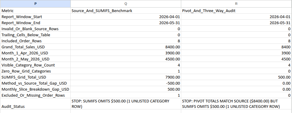
The SUMIFS grid drops to $7,900.00. Nothing on the grid says why, because no row is set up for Training. The pivot adds a Training row with $500.00 in May and keeps the grand total at $8,400.00. Google Sheets updated the pivot as soon as the cell changed. Excel for the web showed the change only after Data > Refresh All. After C8 was changed back and the pivot refreshed, Excel still listed Training in the category filter list.
Dates outside the grid behave the same way. Change B8 to 2026-06-03. May in the grid drops to $4,000.00 and the grid total to $7,900.00. The pivot adds a 2026-06 column with $500.00 and still totals $8,400.00.
You can catch both problems on the SUMIFS side, too. Helper column H marks each row "INCLUDED", "UNLISTED CATEGORY", or "OUT OF GRID MONTHS", so the missing $500.00 points to an exact row. To stop new labels at the source, use dropdowns to keep categories consistent and keep the approved list in a small data dictionary.
How Each Method Gives a Wrong Total
Five more mistakes came out of the test. Start each one from the clean export.
| Mistake | What you see | Where it was tested |
|---|---|---|
| Excel pivot not refreshed after a source edit | Pivot shows $8,100.00 while the source totals $8,400.00 | Excel for the web |
| A category unchecked in the pivot filter | Pivot shows $7,300.00 across 6 orders and 2 categories | Both |
| Dates grouped by month without the year | April shows $3,900.00, though April 2026 is only $2,800.00 | Google Sheets |
| Values summarized by count instead of sum | Pivot shows 4, 4, and 8 instead of dollars | Both |
| A new row added below the ranges | Grid and pivot both show $8,400.00 and both miss $450.00 | Both |
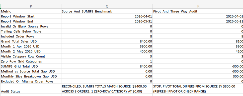
Stale Excel pivot. In the test, D9 was set to 550, the pivot was refreshed to $8,100.00, and then D9 went back to 850 without a refresh. The SUMIFS grid returned to $8,400.00 at once. The pivot stayed at $8,100.00, with May at $4,200.00. The tested Excel for the web workbook had no automatic refresh option, and refresh on opening was turned off in its pivot settings. Google Sheets never reached a stale state because its pivot recalculated on every edit.
Month without the year. Change B2 to 2025-04-10. With Year-Month grouping, Google Sheets split out a 2025-Apr column with $1,100.00 and left 2026-Apr at $2,800.00. With Month grouping, both years merged into one Apr column showing $3,900.00. The grand total stayed at $8,400.00, so the error shows only in the monthly split. In Excel for the web, column E kept 2025-04 separate. It appeared to the right of 2026-05, not before April, so check the column order.
Count instead of sum. If Values summarizes net_sales_usd by count, the pivot shows 4, 4, and 8. Those are order counts that look like small totals.
The new row nobody included. Add ORD-7009 in row 10: 2026-05-30, Installation, $450.00. The grid’s ranges end at row 9, and so does a pivot built on A1:E9. Both still say $8,400.00, and they agree with each other. Matching each other doesn’t make them right.
Check Both Methods Against the Source Rows
The check block sits in P1:R16. Column P holds labels. Column Q calculates each metric from the source rows and the SUMIFS grid. Column R holds five readings you type in from the pivot, plus checks that compare them with column Q.
| Row | Metric (P) | Column Q at baseline | What goes in column R |
|---|---|---|---|
| 2 | Report_Window_Start | 2026-04-01 | Type 2026-04-01 |
| 3 | Report_Window_End | 2026-05-31 | Type 2026-05-31 |
| 4 | Invalid_Or_Blank_Source_Rows | 0 | Type 0 |
| 5 | Trailing_Cells_Below_Table | 0 | Type 0 |
| 6 | Included_Order_Rows | 8 | Order count from the pivot’s grand total |
| 7 | Grand_Total_Sales_USD | 8400.00 | Sales grand total from the pivot |
| 8 | Month_1_Apr_2026_USD | 3900.00 | Pivot’s April 2026 subtotal |
| 9 | Month_2_May_2026_USD | 4500.00 | Pivot’s May 2026 subtotal |
| 10 | Visible_Category_Row_Count | 3 | Number of category labels in the pivot |
| 11 | Zero_Row_Grid_Categories | 1 | Formula: pivot categories minus source categories |
| 12 | SUMIFS_Grid_Total_USD | 8400.00 | Formula: pivot minus grid |
| 13 | Method_vs_Source_Total_Gap_USD | 0.00 | Formula: pivot minus source |
| 14 | Monthly_Slice_Breakdown_Gap_USD | 0.00 | Formula: pivot month gaps |
| 15 | Excluded_Or_Missing_Order_Rows | 0 | Formula: pivot rows minus source rows |
| 16 | Audit_Status | Status message | Status message |
Until you read the pivot, type NOT TESTED in R6:R10. Read R6 from the pivot’s own order count, not from column Q. For R10, count only the category labels between the pivot’s header and its Grand Total row.
Q5 is the guard for new rows. It counts every filled cell in columns A to E and subtracts the cells inside A1:E9: =COUNTA($A:$E)-COUNTA($A$1:$E$9). Anything below row 9, whether in row 10 or row 500, makes it greater than 0.
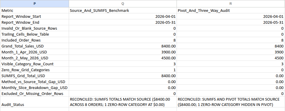
Here’s what the two status cells said in the test:
| Situation | Q16 (source and SUMIFS) | R16 (all three) |
|---|---|---|
| Clean export, pivot read | RECONCILED: SUMIFS TOTALS MATCH SOURCE ($8400.00 ACROSS 8 ORDERS; 1 ZERO-ROW CATEGORY AT $0.00) |
RECONCILED: SUMIFS AND PIVOT TOTALS MATCH SOURCE ($8400.00; 1 ZERO-ROW CATEGORY HIDDEN IN PIVOT) |
Training in C8 |
STOP: SUMIFS OMITS $500.00 (1 UNLISTED CATEGORY ROW) |
STOP: PIVOT TOTALS MATCH SOURCE ($8400.00) BUT SUMIFS OMITS $500.00 (1 UNLISTED CATEGORY ROW) |
| Unrefreshed Excel pivot | Reconciled | STOP: PIVOT TOTAL DIFFERS FROM SOURCE BY $300.00 (REFRESH PIVOT OR CHECK RANGE) |
| Support unchecked | Reconciled | STOP: PIVOT ORDER COUNT MISMATCH (6 VS 8; CHECK FILTERS OR RANGE) |
| Month-only grouping | STOP: SUMIFS OMITS $1100.00 (1 OUT-OF-WINDOW DATE ROW) |
STOP: PIVOT MONTH BREAKDOWN DIFFERS BY $1100.00 (CHECK YEAR-MONTH GROUPING OR SLICE TOTALS) |
| Summarized by count | Reconciled | STOP: PIVOT SUMMARIZES COUNT (8) INSTEAD OF SUM ($8400.00) |
| New row 10 | STOP: TRAILING SOURCE DATA OUTSIDE TABLE RANGE (RESIZE RANGES) |
Same message |
In the stale-pivot case, R13 shows -300.00 because the pivot is $300.00 below the source. The status message drops the sign and reports the size of the gap.
In the month-only case, Q16 also stops, because the 2025 order sits outside the April–May 2026 window. In a real report, that stop is the point: the order belongs to another period.
When Next Month’s Export Changes Size
When the export grows or shrinks, update the formulas and the pivot together. The last row is always the order count plus 1. The example starts with 8 orders, so its last row is 9.
- Enter the orders. When the export grows, type the new orders in columns A to D below the old last row, and leave columns E to I empty in those rows for now. When it shrinks, don’t clear anything yet.
- Replace the old last row with the new one. Select
E2:R16. If the old last row is below row 16, select down to it instead, such asE2:R21. Replace:$A$followed by the old last row with:$A$followed by the new last row. Do the same for columns B through I, so nine replacements in all. Going from 8 orders to 9, that’s:$A$9to:$A$10. Going later from 9 orders to 20, it’s:$A$10to:$A$21. - Fill the helpers. Copy
E2:I2down to the new last row. When the export shrinks, then clear the unused cells in columns A to I only, from the row below the new last row down to the old last row. Don’t delete whole rows, because that would also move or cut the grid and the check block beside the export. - Point the pivot at the new range, such as
A1:E10. In Google Sheets, edit the range in the pivot table editor. In Excel for the web, use PivotTable > Change Data Source. In the test, Refresh All alone didn’t pick up row 10 while the source stayedA1:E9. - Refresh the pivot in Excel.
- Read the pivot again and retype
R6:R10.
For step 2, keep the replacement inside your selection and make it match text inside formulas:
- Google Sheets: Choose Edit > Find and replace, set Search to Specific range with your selection, and check Also search within formulas. Leave Search using regular expressions unchecked, because the $ sign has a special meaning there.
- Excel for the web: Open Replace, expand Search Options, set Within to Selection, and leave Match entire cell contents unchecked (Find or replace text and numbers).
Each replacement must start from the current last row. If you add more orders later and repeat :$A$9 to :$A$10, nothing changes, and Q5 stops the report with STOP: TRAILING SOURCE DATA OUTSIDE TABLE RANGE (RESIZE RANGES). That message tells you the ranges still end above your data.
Going from 8 orders to 9, both statuses reconciled at $8,850.00 across 9 orders after step 6. Installation now had a source row, so the zero-row count dropped to 0. If you stop after step 3 and keep the old readings in R6:R10, R16 says STOP: PIVOT ORDER COUNT MISMATCH (8 VS 9; CHECK FILTERS OR RANGE).
Shrinking works the same way. Going from 8 orders to 5, the last row moves from 9 to 6, so replace :$A$9 with :$A$6 through column I, then clear A7:I9. Growing from 5 orders to 9 later means replacing :$A$6 with :$A$10.
Replace only those nine strings. A broader replace changes references that should stay fixed. After shrinking to 5 orders, for example, replacing every $6 would also change $N$6 in column H. The row-count checks use ROWS($A$2:$A$9), so they update with the same nine replacements. The test ran 8 to 5 to 9, 8 to 4 to 9, 8 to 1 to 9 to 20, and an export of 105 orders, and every chain passed in both programs.
Google Sheets has a shortcut for the pivot side. Enter the source range as Sales_Report!A1:E and add a filter on sale_date with Filter by condition > Is not empty. Sheets saved the range as A1:E1000. The pivot picked up row 10 on its own and dropped it again when the row was cleared. The SUMIFS ranges still need the replacement steps.
In Excel, a pivot built on a formatted table includes new table rows when you refresh it (Create a PivotTable). The formulas in this workbook use fixed cell ranges, though, so formatting the export as a table doesn’t change them. This article uses plain ranges so the same steps work in both programs.
What These Checks Can’t Prove
The check compares five totals and counts. It doesn’t compare each category cell. Suppose D2 (April Hardware) rises from 1,100 to 1,200 and D3 (April Software) falls from 1,500 to 1,400. The order count, both month totals, and the grand total stay the same. In the test, an unrefreshed Excel pivot still showed Hardware at $1,800.00 while the grid showed $1,900.00, and R16 still said reconciled. Refresh every Excel pivot before you share it, even when the check passes.
The check also can’t tell you whether an order was missing from the export. It only shows that the rows on the sheet were summed the same way three times. Compare the order count in Q6 and the total in Q7 with the count and sales total from your billing or point-of-sale system, for the same dates and currency.
Frequently Asked Questions
Can you use a pivot table and SUMIFS in the same monthly report?
Yes, and it often works best. Use the pivot table to scan each new export for unexpected labels and months. Then let the SUMIFS grid feed the report that other sheets depend on. Column H and Q16 tell you if the grid skipped anything.
Why use EDATE instead of EOMONTH for the month’s end?
Some exports include the time of the sale. If the $600.00 Support order is stamped 2026-04-30 14:30, a bare SUMIFS with "<"&EDATE(L$1, 1) still counts it, and April totals $3,900.00. With "<="&EOMONTH(L$1, 0), the cutoff is midnight at the start of April 30, so the order drops out, and April shows $3,300.00. In the full workbook, helper column F marks a timestamped row "CHECK ROW" and stops the report, so convert timestamps to plain dates before you paste the export.
Should I use a table instead of a plain range?
In Excel, a table can save you the pivot’s resize step, because a pivot built on the table picks up new rows when you refresh it. The formulas are a different matter. You’d have to rewrite them with structured references, then adapt and retest the checks. In Google Sheets, pivot tables don’t currently accept table references (Use table references), so the open range above is the practical option. Whatever you use, keep every range in one SUMIFS the same height. In Excel, mismatched ranges return #VALUE! (SUMIFS function).
What to Do Next
Pick the method by what reads the report. If formulas downstream need fixed rows, use SUMIFS and check it against a pivot each month. If you’re still learning what the export contains, start with a pivot. Either way, run the three-way check before you share. If your report combines a new file every month, also confirm that the report included the new month.
Formula Reference
Each label before = names the destination cell; paste only the formula. Fill E2:I2 down to row 9. Enter L2 and fill it to L2:M5. Fill N2 down to N5 and L6 across to M6. Paste the column Q and R formulas one cell at a time.
Typed inputs: L1 = 2026-04-01, M1 = 2026-05-01, Q2 and R2 = 2026-04-01, Q3 and R3 = 2026-05-31, R4 and R5 = 0. Put NOT TESTED in R6:R10 until you read the pivot.
Source helpers:
E2: =IF(NOT(EXACT(F2, "OK")), "", TEXT(B2, "yyyy-mm"))
F2: =IF(OR(COUNTA(A2:D2)<4, NOT(ISTEXT(A2)), NOT(ISNUMBER(B2)), NOT(ISTEXT(C2)), NOT(ISNUMBER(D2)), TRIM(SUBSTITUTE(A2, CHAR(160), " "))="", TRIM(SUBSTITUTE(C2, CHAR(160), " "))="", NOT(EXACT(A2, TRIM(SUBSTITUTE(A2, CHAR(160), " ")))), NOT(EXACT(C2, TRIM(SUBSTITUTE(C2, CHAR(160), " ")))), NOT(EXACT(A2, UPPER(A2))), NOT(EXACT(C2, PROPER(C2))), NOT(ISERROR(FIND(" ", A2&C2))), NOT(ISERROR(FIND("*", A2&C2))), NOT(ISERROR(FIND("?", A2&C2))), NOT(ISERROR(FIND("~", A2&C2))), NOT(ISERROR(FIND("=", A2&C2))), NOT(ISERROR(FIND("<", A2&C2))), NOT(ISERROR(FIND(">", A2&C2)))), "CHECK ROW", IF(OR(INT(B2)<>B2, B2<DATE(2000,1,1), B2>DATE(2100,1,1), D2<0, ROUND(D2, 2)<>D2), "CHECK ROW", "OK"))
G2: =IF(OR(NOT(EXACT(F2, "OK")), COUNTIF($F$2:$F$9, "OK")<ROWS($A$2:$A$9)), "", SUMPRODUCT(--EXACT($A$2:$A$9, A2)))
H2: =IF(OR(NOT(EXACT(F2, "OK")), NOT(ISNUMBER($N$6))), "CHECK INPUTS", IF(SUMPRODUCT(--EXACT($K$2:$K$5, C2))=0, "UNLISTED CATEGORY", IF(OR(B2<$L$1, B2>=EDATE($M$1, 1)), "OUT OF GRID MONTHS", "INCLUDED")))
I2: =IF(OR(NOT(EXACT(F2, "OK")), COUNT($G$2:$G$9)<ROWS($A$2:$A$9)), "", IF(SUMPRODUCT(--EXACT($C$2:C2, C2))=1, 1, 0))
SUMIFS grid:
L2: =IF(OR(COUNTIF($F$2:$F$9, "OK")<ROWS($A$2:$A$9), COUNT($G$2:$G$9)<ROWS($A$2:$A$9), COUNTIF($G$2:$G$9, ">1")>0, NOT(ISTEXT($K2)), TRIM(SUBSTITUTE($K2, CHAR(160), " "))="", NOT(EXACT($K2, TRIM(SUBSTITUTE($K2, CHAR(160), " ")))), NOT(EXACT($K2, PROPER($K2))), NOT(ISERROR(FIND(" ", $K2))), NOT(ISERROR(FIND("*", $K2))), NOT(ISERROR(FIND("?", $K2))), NOT(ISERROR(FIND("~", $K2))), NOT(ISERROR(FIND("=", $K2))), NOT(ISERROR(FIND("<", $K2))), NOT(ISERROR(FIND(">", $K2))), SUMPRODUCT(--EXACT($K$2:$K$5, $K2))>1, NOT(ISNUMBER(L$1)), NOT(ISNUMBER($L$1)), NOT(ISNUMBER($M$1)), NOT(ISNUMBER($Q$2)), NOT(ISNUMBER($Q$3))), "CHECK INPUTS", IF(OR(INT(L$1)<>L$1, DAY(L$1)<>1, L$1<DATE(2000,1,1), L$1>DATE(2100,1,1), COUNTIF($L$1:$M$1, L$1)>1, INT($L$1)<>$L$1, INT($M$1)<>$M$1, INT($Q$2)<>$Q$2, INT($Q$3)<>$Q$3, $L$1<>$Q$2, $M$1<>EDATE($L$1, 1), $Q$3<>EOMONTH($M$1, 0)), "CHECK INPUTS", ROUND(SUMIFS($D$2:$D$9, $C$2:$C$9, $K2, $B$2:$B$9, ">="&L$1, $B$2:$B$9, "<"&EDATE(L$1, 1)), 2)))
N2: =IF(COUNT(L2:M2)<2, "CHECK INPUTS", ROUND(SUM(L2:M2), 2))
L6: =IF(COUNT(L2:L5)<4, "CHECK INPUTS", ROUND(SUM(L2:L5), 2))
N6: =IF(OR(COUNT(L6:M6)<2, COUNT(N2:N5)<4), "CHECK INPUTS", IF(ROUND(SUM(L6:M6)-SUM(N2:N5), 2)<>0, "CHECK CROSS-FOOT", ROUND(SUM(N2:N5), 2)))
Source and SUMIFS checks:
Q4: =COUNTIF($F$2:$F$9, "<>OK")+COUNTBLANK($A$2:$A$9)+COUNTBLANK($B$2:$B$9)+COUNTBLANK($C$2:$C$9)+COUNTBLANK($D$2:$D$9)
Q5: =COUNTA($A:$E)-COUNTA($A$1:$E$9)
Q6: =IF(OR(Q4>0, Q5>0, COUNT($G$2:$G$9)<ROWS($A$2:$A$9), COUNT($I$2:$I$9)<ROWS($A$2:$A$9), NOT(ISNUMBER(N6))), "CHECK INPUTS", COUNTA($A$2:$A$9))
Q7: =IF(NOT(ISNUMBER(Q6)), "CHECK INPUTS", ROUND(SUM($D$2:$D$9), 2))
Q8: =IF(NOT(ISNUMBER(Q6)), "CHECK INPUTS", ROUND(SUMIFS($D$2:$D$9, $B$2:$B$9, ">="&$L$1, $B$2:$B$9, "<"&EDATE($L$1, 1)), 2))
Q9: =IF(NOT(ISNUMBER(Q6)), "CHECK INPUTS", ROUND(SUMIFS($D$2:$D$9, $B$2:$B$9, ">="&$M$1, $B$2:$B$9, "<"&EDATE($M$1, 1)), 2))
Q10: =IF(NOT(ISNUMBER(Q6)), "CHECK INPUTS", SUM($I$2:$I$9))
Q11: =IF(NOT(ISNUMBER(Q6)), "CHECK INPUTS", IF(COUNTIF($C$2:$C$9, K2)=0, 1, 0)+IF(COUNTIF($C$2:$C$9, K3)=0, 1, 0)+IF(COUNTIF($C$2:$C$9, K4)=0, 1, 0)+IF(COUNTIF($C$2:$C$9, K5)=0, 1, 0))
Q12: =IF(NOT(ISNUMBER(Q6)), "CHECK INPUTS", ROUND(N6, 2))
Q13: =IF(NOT(ISNUMBER(Q6)), "CHECK INPUTS", ROUND(Q12-Q7, 2))
Q14: =IF(NOT(ISNUMBER(Q6)), "CHECK INPUTS", ROUND(ABS(L6-Q8)+ABS(M6-Q9), 2))
Q15: =IF(OR(NOT(ISNUMBER(Q6)), COUNTIF($H$2:$H$9, "CHECK INPUTS")>0), "CHECK INPUTS", COUNTIF($H$2:$H$9, "<>INCLUDED"))
Q16: =IF(Q4>0, "STOP: INVALID OR BLANK SOURCE ROWS", IF(COUNTIF($G$2:$G$9, ">1")>0, "STOP: DUPLICATE ORDER IDS IN SOURCE", IF(Q5>0, "STOP: TRAILING SOURCE DATA OUTSIDE TABLE RANGE (RESIZE RANGES)", IF(NOT(ISNUMBER(N6)), "STOP: CHECK SUMIFS GRID HEADERS OR DATES", IF(NOT(ISNUMBER(Q6)), "STOP: CHECK SOURCE INPUTS", IF(AND(COUNTIF($H$2:$H$9, "UNLISTED CATEGORY")>0, COUNTIF($H$2:$H$9, "OUT OF GRID MONTHS")>0), "STOP: SUMIFS OMITS $" & TEXT(ABS(Q13), "0.00") & " (" & Q15 & " UNLISTED CATEGORY AND OUT-OF-WINDOW ROWS)", IF(COUNTIF($H$2:$H$9, "UNLISTED CATEGORY")>0, "STOP: SUMIFS OMITS $" & TEXT(ABS(Q13), "0.00") & " (" & Q15 & IF(Q15=1, " UNLISTED CATEGORY ROW)", " UNLISTED CATEGORY ROWS)"), IF(COUNTIF($H$2:$H$9, "OUT OF GRID MONTHS")>0, "STOP: SUMIFS OMITS $" & TEXT(ABS(Q13), "0.00") & " (" & Q15 & IF(Q15=1, " OUT-OF-WINDOW DATE ROW)", " OUT-OF-WINDOW DATE ROWS)"), IF(OR(Q13<>0, Q14<>0, Q15<>0), "STOP: SUMIFS DIFFERS FROM SOURCE BY $" & TEXT(ABS(Q13), "0.00"), "RECONCILED: SUMIFS TOTALS MATCH SOURCE ($" & TEXT(Q7, "0.00") & " ACROSS " & Q6 & " ORDERS; " & Q11 & IF(Q11=1, " ZERO-ROW CATEGORY AT $0.00)", " ZERO-ROW CATEGORIES AT $0.00)"))))))))))
Pivot checks:
R11: =IF(EXACT(R15, "NOT TESTED"), "NOT TESTED", IF(OR(NOT(ISNUMBER(R15)), NOT(ISNUMBER(Q10)), NOT(ISNUMBER(R10))), "CHECK INPUTS", R10-Q10))
R12: =IF(EXACT(R15, "NOT TESTED"), "NOT TESTED", IF(OR(NOT(ISNUMBER(R15)), NOT(ISNUMBER(Q12)), NOT(ISNUMBER(R7))), "CHECK INPUTS", ROUND(R7-Q12, 2)))
R13: =IF(EXACT(R15, "NOT TESTED"), "NOT TESTED", IF(OR(NOT(ISNUMBER(R15)), NOT(ISNUMBER(Q7)), NOT(ISNUMBER(R7))), "CHECK INPUTS", ROUND(R7-Q7, 2)))
R14: =IF(EXACT(R15, "NOT TESTED"), "NOT TESTED", IF(OR(NOT(ISNUMBER(R15)), NOT(ISNUMBER(Q8)), NOT(ISNUMBER(Q9)), NOT(ISNUMBER(R8)), NOT(ISNUMBER(R9))), "CHECK INPUTS", ROUND(ABS(R8-Q8)+ABS(R9-Q9), 2)))
R15: =IF(OR(Q4>0, Q5>0, COUNTIF($G$2:$G$9, ">1")>0, NOT(ISNUMBER(Q6)), NOT(ISNUMBER(Q15)), NOT(ISNUMBER(R2)), NOT(ISNUMBER(R3)), NOT(ISNUMBER(R4)), NOT(ISNUMBER(R5))), "CHECK INPUTS", IF(OR(INT(R2)<>R2, INT(R3)<>R3, R2<>Q2, R3<>Q3, INT(R4)<>R4, R4<>0, INT(R5)<>R5, R5<>0), "CHECK INPUTS", IF(AND(EXACT(R6, "NOT TESTED"), EXACT(R7, "NOT TESTED"), EXACT(R8, "NOT TESTED"), EXACT(R9, "NOT TESTED"), EXACT(R10, "NOT TESTED")), "NOT TESTED", IF(OR(NOT(ISNUMBER(R6)), NOT(ISNUMBER(R7)), NOT(ISNUMBER(R8)), NOT(ISNUMBER(R9)), NOT(ISNUMBER(R10))), "CHECK INPUTS", IF(OR(INT(R6)<>R6, R6<0, R7<0, ROUND(R7, 2)<>R7, R8<0, ROUND(R8, 2)<>R8, R9<0, ROUND(R9, 2)<>R9, INT(R10)<>R10, R10<0), "CHECK INPUTS", R6-Q6)))))
R16: =IF(Q4>0, "STOP: INVALID OR BLANK SOURCE ROWS", IF(COUNTIF($G$2:$G$9, ">1")>0, "STOP: DUPLICATE ORDER IDS IN SOURCE", IF(Q5>0, "STOP: TRAILING SOURCE DATA OUTSIDE TABLE RANGE (RESIZE RANGES)", IF(NOT(ISNUMBER(N6)), "STOP: CHECK SUMIFS GRID HEADERS OR DATES", IF(IF(AND(ISNUMBER(R2), ISNUMBER(R3)), OR(INT(R2)<>R2, INT(R3)<>R3, R2<>Q2, R3<>Q3), TRUE), "STOP: REPORT WINDOW MISMATCH", IF(IF(AND(ISNUMBER(R4), ISNUMBER(R5)), OR(INT(R4)<>R4, R4<>0, INT(R5)<>R5, R5<>0), TRUE), "STOP: INVALID AUDIT GUARD INPUTS", IF(EXACT(R15, "NOT TESTED"), "NOT TESTED: ENTER PIVOT TABLE READINGS", IF(EXACT(R15, "CHECK INPUTS"), "STOP: NON-NUMERIC, NEGATIVE, OR INCOMPLETE PIVOT INPUTS", IF(AND(Q7<>Q6, R7=Q6, ROUND(R8+R9, 2)=Q6), "STOP: PIVOT SUMMARIZES COUNT (" & Q6 & ") INSTEAD OF SUM ($" & TEXT(Q7, "0.00") & ")", IF(R15<>0, "STOP: PIVOT ORDER COUNT MISMATCH (" & R6 & " VS " & Q6 & "; CHECK FILTERS OR RANGE)", IF(R13<>0, "STOP: PIVOT TOTAL DIFFERS FROM SOURCE BY $" & TEXT(ABS(R13), "0.00") & " (REFRESH PIVOT OR CHECK RANGE)", IF(R14>0, "STOP: PIVOT MONTH BREAKDOWN DIFFERS BY $" & TEXT(R14, "0.00") & " (CHECK YEAR-MONTH GROUPING OR SLICE TOTALS)", IF(R11<>0, "STOP: PIVOT VISIBLE CATEGORY COUNT MISMATCH (" & R10 & " VS " & Q10 & ")", IF(AND(COUNTIF($H$2:$H$9, "UNLISTED CATEGORY")>0, COUNTIF($H$2:$H$9, "OUT OF GRID MONTHS")>0), "STOP: PIVOT TOTALS MATCH SOURCE ($" & TEXT(Q7, "0.00") & ") BUT SUMIFS OMITS $" & TEXT(ABS(Q13), "0.00") & " (" & Q15 & " UNLISTED CATEGORY AND OUT-OF-WINDOW ROWS)", IF(COUNTIF($H$2:$H$9, "UNLISTED CATEGORY")>0, "STOP: PIVOT TOTALS MATCH SOURCE ($" & TEXT(Q7, "0.00") & ") BUT SUMIFS OMITS $" & TEXT(ABS(Q13), "0.00") & " (" & Q15 & IF(Q15=1, " UNLISTED CATEGORY ROW)", " UNLISTED CATEGORY ROWS)"), IF(COUNTIF($H$2:$H$9, "OUT OF GRID MONTHS")>0, "STOP: PIVOT TOTALS MATCH SOURCE ($" & TEXT(Q7, "0.00") & ") BUT SUMIFS OMITS $" & TEXT(ABS(Q13), "0.00") & " (" & Q15 & IF(Q15=1, " OUT-OF-WINDOW DATE ROW)", " OUT-OF-WINDOW DATE ROWS)"), IF(OR(Q13<>0, Q14<>0, Q15<>0), "STOP: SUMIFS DIFFERS FROM SOURCE BY $" & TEXT(ABS(Q13), "0.00"), "RECONCILED: SUMIFS AND PIVOT TOTALS MATCH SOURCE ($" & TEXT(Q7, "0.00") & "; " & Q11 & IF(Q11=1, " ZERO-ROW CATEGORY HIDDEN IN PIVOT)", " ZERO-ROW CATEGORIES HIDDEN IN PIVOT)"))))))))))))))))))