
Only average a 1-to-5 customer rating when you state upfront that you are treating the steps between scores as equal, and report the median plus the 1-to-2 and 4-to-5 score shares alongside that average. Never average numbers that only label categories like postal zones or unordered outcome codes because changing those arbitrary code digits moves the average even when customer results stay the same.
In the 15-response feedback export below, each of the three branches has 5 completed surveys. South averages 3.40 (17 divided by 5) ahead of North at 3.20 (16 divided by 5), while the median flips their order to 3.00 for South versus 4.00 for North. Two 1-star ratings from cancelled parts backorders pull North’s mean down even though 60% of North’s responses (3 of 5) are 4 or 5, whereas West leads on both measures with a 4.60 mean and a 5.00 median. Five responses per branch describe only this small batch of responses, not a permanent ranking of branch performance.
This is the second companion article in Grain First, my open-core data analytics curriculum, following Why Counting Rows Can Mislead You: Row Grain vs. Unit of Analysis. You can try the live Level 1 and Level 2 interactive practice exercises for this unit on CareerTalkLab while the walkthrough video is still being recorded, and business owners checking their own reporting can start with the 4-Minute Small Business Data Audit.
I’ve seen business numbers that should agree fall out of sync across software systems plenty of times. My preferred tool is Google Sheets because a spreadsheet should be shareable. It should make collaborating with others easy. Every formula in this walkthrough returns the same results in Google Sheets and Excel for the web with US English settings.
Below is the 15-row customer feedback export I made up for this article.
| Row | response_id (A) | branch (B) | response_date (C) | postal_district (D) | outcome_code (E) | rating_1_to_5 (F) | invoice_usd (G) |
|---|---|---|---|---|---|---|---|
| 2 | RSP-01 | North | 2026-10-01 | 410 | 1 | 5 | 200.00 |
| 3 | RSP-02 | North | 2026-10-02 | 420 | 4 | 1 | 0.00 |
| 4 | RSP-03 | North | 2026-10-03 | 435 | 2 | 4 | 180.00 |
| 5 | RSP-04 | North | 2026-10-04 | 455 | 1 | 5 | 220.00 |
| 6 | RSP-05 | North | 2026-10-05 | 480 | 4 | 1 | 0.00 |
| 7 | RSP-06 | South | 2026-10-01 | 410 | 1 | 3 | 110.00 |
| 8 | RSP-07 | South | 2026-10-02 | 420 | 2 | 4 | 120.00 |
| 9 | RSP-08 | South | 2026-10-03 | 435 | 3 | 3 | 100.00 |
| 10 | RSP-09 | South | 2026-10-04 | 455 | 1 | 3 | 110.00 |
| 11 | RSP-10 | South | 2026-10-05 | 480 | 3 | 4 | 110.00 |
| 12 | RSP-11 | West | 2026-10-01 | 410 | 1 | 5 | 130.00 |
| 13 | RSP-12 | West | 2026-10-02 | 420 | 2 | 4 | 120.00 |
| 14 | RSP-13 | West | 2026-10-03 | 435 | 1 | 5 | 140.00 |
| 15 | RSP-14 | West | 2026-10-04 | 455 | 2 | 4 | 120.00 |
| 16 | RSP-15 | West | 2026-10-05 | 480 | 2 | 5 | 140.00 |
In the spreadsheet walkthrough below, these seven columns sit in columns A through G on rows 2 to 16; the Row column above is for reading reference only and is left out when pasting. One row records one completed post-service feedback survey, with a unique identifier in response_id. The postal_district column uses fictional 3-digit zones (410, 420, 435, 455, and 480) rather than real US ZIP codes. The outcome_code column assigns digits 1 to 4 to unordered outcomes: 1 means completed in-store (6 rows, 40.0%), 2 means completed by mobile van (5 rows, 33.3%), 3 means referred to a partner shop (2 rows, 13.3%), and 4 means a cancelled parts backorder with $0.00 billed (2 rows, 13.3%). Ratings run from 1 (Very Dissatisfied) to 5 (Very Satisfied), where a blank cell means missing rather than zero, and invoice_usd tracks billed revenue in US dollars.
Here are the branch rollups computed from those 15 rows (shares appear as two-decimal percentages alongside four-decimal proportions, and ratings appear to two decimals):
| Branch | Responses | Bottom-2-Box (1–2) |
Top-2-Box (4–5) |
rating_mean |
rating_median |
Mean Rank | Median Rank | What the Numbers Show |
|---|---|---|---|---|---|---|---|---|
| North | 5 | 40.00% (0.4000) | 60.00% (0.6000) | 3.20 | 4.00 | 3 | 2 | Polarized: two 1-star cancelled backorders ($0.00 billed) vs. three 4-to-5 visits |
| South | 5 | 0.00% (0.0000) | 40.00% (0.4000) | 3.40 | 3.00 | 2 | 3 | Lukewarm: zero 1-to-2 ratings, three 3-star visits, and two 4-star visits |
| West | 5 | 0.00% (0.0000) | 100.00% (1.0000) | 4.60 | 5.00 | 1 | 1 | Aligned: 100.00% 4-to-5 ratings, no 1-to-2 scores, rank 1 on both mean and median |
| All_Branches | 15 | 13.33% (0.1333) | 66.67% (0.6667) | 3.73 | 4.00 | N/A | N/A | Rank flip present across 2 of 3 branches |
The rightmost column above summarizes each row in plain English; Step 2 builds the worksheet’s automated scale_guidance flags in column S.
The Two Opposite Rating-Scale Mistakes
Picture a hypothetical weekly operations meeting where one person drops this export into a pivot summary and another refuses to let anyone summarize ratings with an average. Both habits break weekly reporting in opposite ways.
- Credulous averaging (the nominal trap): Running
=AVERAGE(E2:E16)onoutcome_codereturns 2.00 (“Completed by mobile van”), even though code 1 (“Completed in-store”) is the most common outcome at 40.0%. Re-number code 4 (“Parts backorder cancelled”) to 9, and=AVERAGE(E2:E16)jumps from 2.00 to 2.67 without changing a single visit. Running=AVERAGE(D2:D16)onpostal_districtreturns 440.00, and changing zone 480 to 900 pushes that mean to 524.00. An unobserved mean value is not the flaw by itself, since averaging two valid invoices of $100.00 and $150.00 produces a valid $125.00 mean even though neither invoice equals $125.00. What fails on nominal labels is running magnitude-based math (AVERAGE,SUM, or numeric rank comparisons) on arbitrary code digits, whereas running Google Sheets MODE or Excel MODE.SNGL onoutcome_codepreserves the modal category (code 1 with 6 occurrences) under one-to-one relabeling. - Dogmatic refusal: Banning every 1-to-5 rating average creates the opposite trap. On West’s clean unimodal scores (5, 4, 5, 4, 5), both the 4.60 mean and the 5.00 median place West first, with 100.00% of scores at 4 or 5 and 0.00% at 1 or 2. More practically, two unimodal branches often tie on the median: a branch with ratings
[4, 4, 4, 4, 5](mean 4.20) and a branch with[3, 4, 4, 4, 4](mean 3.80) both have a median of 4.00. As noted in UCLA OARC’s guide to variable measurement levels and OpenStax Introductory Statistics 2e Section 1.3, ordered survey choices do not guarantee equal psychological steps between 1 and 2 versus 4 and 5. Stating the equal-step assumption when you report a rating mean is a practical reporting convention, not proof of equal psychological distance, and pairing that mean with the median and low/high score shares stops polarized scores like North from getting hidden.
Why Odd-Count and Even-Count Medians Behave Differently
With an odd number of ratings per branch (5 rows per branch and 15 rows overall here), Google Sheets MEDIAN and Microsoft Excel MEDIAN return one observed response at the center of the sorted list. Because no averaging occurs between adjacent scores on odd counts, any strictly increasing relabeling preserves the middle category and the ordering between branches.
When a branch has an even number of responses and its two center positions differ, standard spreadsheet MEDIAN returns their arithmetic midpoint. More generally, Google Sheets PERCENTILE and Excel PERCENTILE.INC apply numeric interpolation at fractional rank positions, which can interpolate even on odd sample counts whenever the requested percentile falls between two observations (Google’s notes specifically single out the 50th percentile as equivalent to MEDIAN).
Under strictly increasing nonlinear relabelings, preserving ties or rankings on interpolated even-count medians is not guaranteed. Suppose Branch A has 6 ratings [1, 1, 1, 5, 5, 5] and Branch B has [3, 3, 3, 3, 3, 3]. Spreadsheet MEDIAN returns 3.00 for both, even though nobody in Branch A picked 3 (its two middle categories are 1 and 5). If you square every score (f(x) = x^2), Branch B keeps a median of 9.00, while Branch A’s midpoint jumps to 13.00 ((1 + 25) / 2). Keep conventional spreadsheet MEDIAN for cross-team compatibility, and on even sample sizes pair it with 1-to-2 and 4-to-5 score shares or list the two middle categories whenever they differ.
Classify Every Column Before You Summarize It
Before calculating a single summary, map every column to its measurement scale, just as you would when building a simple data dictionary (Build a Small Data Dictionary for Your Spreadsheet). Spreadsheet formulas happily add or average any cell containing digits, whether those digits represent dollars, calendar serials, or branch codes.
| Scale | What Numbers Preserve | Valid Summaries | What Breaks | Columns in Export |
|---|---|---|---|---|
| Nominal | Identity and category membership only | Counts, % shares, MODE / MODE.SNGL |
AVERAGE, SUM, magnitude rank |
response_id, branch, postal_district, outcome_code |
| Ordinal | Rank order without guaranteed equal steps | Counts, Bottom-2-Box, Top-2-Box, MEDIAN (note midpoint on even counts), equal-step-disclosed mean |
SUM, unconditional mean without shares/assumption, assuming ties survive nonlinear recodes on interpolated even-count medians |
rating_1_to_5 |
| Interval | Equal spacing without a true zero | MIN, MAX, span (MAX - MIN), AVERAGE (mean date) |
SUM (694,470 date serials), ratio claims ("twice as recent") |
response_date |
| Ratio | Equal spacing plus a true zero ($0.00 = none) |
SUM ($1,800.00), AVERAGE ($120.00), MEDIAN ($120.00), ratios |
Nothing from scale rules alone (still inspect skew) | invoice_usd |
Three classic spreadsheet traps show why column classification saves hours of cleanup later:
- Dates look numeric inside spreadsheet storage: In Google Sheets and Excel,
2026-10-01is stored as serial number 46296. Running=SUM(C2:C16)returns 694,470, which measures nothing because dates have no true zero point. Summarizeresponse_datewithMIN(2026-10-01),MAX(2026-10-05), and the 4-day span. By contrast,invoice_usdis a true ratio variable ($0.00 literally means zero dollars billed on a cancelled backorder), so $1,800.00 total revenue and $120.00 mean revenue per response require zero extra assumptions. - Typing zero for a missing rating corrupts the denominator: Both Excel AVERAGE and Google Sheets AVERAGE skip blank cells while including zeros in the divisor, which I cover in Blank or Zero: Why Missing Values Change Your Average. Adding two non-responses coded as 0 drags this dataset’s overall rating mean from 3.73 (56 ÷ 15) down to 3.29 (56 ÷ 17), a 0.44-point drop caused by a score that does not exist on the form.
- Equal branch counts hide weighting rules: Each branch here happens to have 5 responses, so averaging the three branch means (3.20, 3.40, 4.60) gives the same 3.73 as dividing total stars (56) by total responses (15). Once branch volumes differ, averaging branch averages weights small and large branches equally, the same denominator trap explained in Why You Should Not Average Margin Percentages. Always divide total rating points by total responses across the raw rows, or weight each branch mean by its response count, as the audit sheet does below.
Good metrics should drive operational decisions that protect revenue, improve efficiency, or cut cost, and on small slices they show what to check first rather than proving a cause. Debating whether South’s 3.40 beats North’s 3.20 misses what the score shares surface in these five-response batches: North’s three completed visits scored 4 or 5 ($180.00 to $220.00 billed), while its two 1-star responses were both cancelled parts backorders billed at $0.00 (40.00% low-score share). Five responses per branch cannot establish a branch-wide cause or prescribe a fix, so treat both patterns as investigation leads: check parts backorder records at North, and review the visit notes behind South’s three 3-star responses before reading more into the branch averages.
Build the Side-by-Side Rating Audit in Google Sheets and Excel
This single-sheet layout (Feedback) keeps the raw survey extract in A1:I16, the branch summary and rank-flip check in K1:S5, and the verified benchmark plus candidate report audit in U1:W15, separated by blank spacer columns J and T. Because K1:S5 ends on row 5 and U1:W15 ends on row 15, resizing the raw table never collides with neighboring audit cells.
Before You Paste: Input Rules and Real-Export Mapping
Follow these rules before dropping a real export into A1:G16 so your validation column stays green:
- Name the worksheet
Feedback, paste only columnsA:G, and leave out the preview’sRowcolumn. - Re-key platform survey IDs into
RSP-01throughRSP-999("RSP-"followed by two or three digits, uppercase, with no spaces, non-breaking spaces, line breaks, or* ? ~ = < >) and keep a lookup crosswalk back to your raw system IDs (Map Inconsistent Customer Names to Stable IDs in Excel and Google Sheets).Row_Check(H2) flags those specific issues; it won’t catch every hidden character. - Map your own branch names to three distinct labels in both
B2:B16andK2:K4, keeping a side crosswalk if your source names contain spaces (for example, mapping"North Shop"toNorth_Shopin both columnBandK2:K4). Every branch label in columnBandK2:K4must match case-sensitively, have at least one valid response (L2:L4 >= 1), and contain no spaces (even when columnBandK2:K4match), non-breaking spaces, line breaks, or* ? ~ = < >becauseRow_Check(H2) rejects all of those characters. This worksheet layout compares exactly three populated branches ($K$2:$K$4, rows 2 to 4, withAll_Brancheson row 5); comparing two branches or four or more branches requires rebuilding the branch summary table, which this walkthrough does not cover. - Enter
response_date(C2:C16) and the window dates (V2:V3,W2:W3) as whole numeric spreadsheet dates (no timestamps) between 2000-01-01 and 2100-01-01, with every response falling insideV2throughV3. If you import an.xlsxfile into Google Sheets, checkFile > Settingsto confirm US English locale (United States) and your expected timezone. - Keep
postal_districtas an integer from 100 to 99999,outcome_codeas an integer from 1 to 4,rating_1_to_5as an integer from 1 to 5, andinvoice_usdzero or higher with no more than two decimal places.
Step 1: Load the Raw Export, Static Controls, and Row Checks
Copy this tab-separated dataset and paste it starting at Feedback!A1 so A1:G16 is populated:
response_id	branch	response_date	postal_district	outcome_code	rating_1_to_5	invoice_usd
RSP-01	North	2026-10-01	410	1	5	200.00
RSP-02	North	2026-10-02	420	4	1	0.00
RSP-03	North	2026-10-03	435	2	4	180.00
RSP-04	North	2026-10-04	455	1	5	220.00
RSP-05	North	2026-10-05	480	4	1	0.00
RSP-06	South	2026-10-01	410	1	3	110.00
RSP-07	South	2026-10-02	420	2	4	120.00
RSP-08	South	2026-10-03	435	3	3	100.00
RSP-09	South	2026-10-04	455	1	3	110.00
RSP-10	South	2026-10-05	480	3	4	110.00
RSP-11	West	2026-10-01	410	1	5	130.00
RSP-12	West	2026-10-02	420	2	4	120.00
RSP-13	West	2026-10-03	435	1	5	140.00
RSP-14	West	2026-10-04	455	2	4	120.00
RSP-15	West	2026-10-05	480	2	5	140.00
Enter all static headers and starting control inputs before pasting live formulas so every check calculates cleanly on first pass:
- Helper headers (
H1:I1): EnterRow_CheckinH1andResponse_ID_FreqinI1. - Branch table frame (
K1:S1andK2:K5): Putbranch,responses,bottom_2_box_share,top_2_box_share,rating_mean,rating_median,mean_rank,median_rank, andscale_guidanceacrossK1:S1, then enterNorth,South,West, andAll_BranchesinK2:K5(or enter your own three distinct, space-free branch labels inK2:K4plusAll_BranchesinK5when loading your own three-branch data). - Audit table frame (
U1:W1,U2:U15): PutCheck_Item,Verified_Sheet_Benchmark, andCandidate_Summary_AuditacrossU1:W1, then enter these exact row labels downU2:U15:Window_Start_Date,Window_End_Date,Audited_Column,Measurement_Scale,Proposed_Summary,Equal_Step_Assumption_Stated,Invalid_Or_Trailing_Cell_Count,Valid_Response_Count,Total_Invoice_USD,Overall_Rating_Mean,Overall_Rating_Median,Rank_Flip_Branch_Count,Reconciliation_Gap, andAudit_Verdict. - Static benchmark controls (
V2:V4,V7): Enter=DATE(2026,10,1)inV2and=DATE(2026,10,5)inV3(formattedyyyy-mm-dd), enterrating_1_to_5inV4, and enterNOinV7. - Starting candidate cells (
W2:W13): Enter=DATE(2026,10,1)inW2and=DATE(2026,10,5)inW3(formattedyyyy-mm-dd),0inW8, andNOT TESTEDinW4:W7andW9:W13.
Now paste the H2 validation formula from the reference section into H2 and fill down through H16, then paste I2 and fill down through I16. All 15 rows return "OK" in H2:H16, and EXACT (Google Sheets, Excel) inside SUMPRODUCT (Google Sheets, Excel) returns 1 down I2:I16. Anytime any row in H2:H16 is not "OK", I2:I16 intentionally stay blank ("") so bad rows cannot quietly leak into branch rollups.
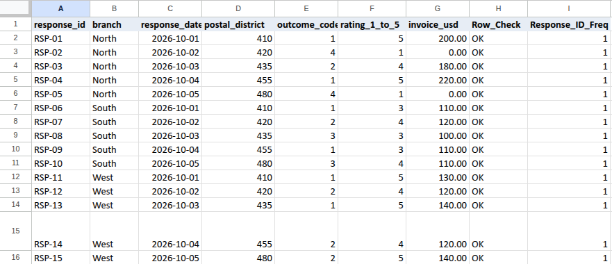
Step 2: Build the Branch Comparison and Rank-Flip Table
Paste each formula from L2 through S2 in the reference section into cells L2:S2 of the branch table and fill L2:S2 down through row 4 (North, South, West), then paste the corresponding formulas into L5:S5 (All_Branches):
- Shares, mean, and cumulative median (
M2:P5): FormatM2:N5as 0.0000 or 0.00% andO2:P5as 0.00, keeping the underlying formulas unrounded so larger exports do not fail exact integer count checks.P2:P4count how many ratings for each branch fall at or below 1, 2, 3, and 4 usingINT((L2+1)/2)andINT((L2+2)/2). That avoids legacyCtrl+Shift+Enterarray formulas (MEDIAN(IF(...))) while matching standard spreadsheetMEDIANon both odd counts (4.00, 3.00, 5.00) and even counts (middle-two midpoint). - Full-precision ranking (
Q2:R4andS2:S5):Q2ranks unrounded means (O2:O4), whileR2ranks medians (P2:P4). KeepingM2:P5unrounded preventsQ2from creating false 0.01-rounded ties between different branch averages such as 23 ÷ 7 (3.2857…) and 56 ÷ 17 (3.2941…) that both display as 3.29, while exact rational ties still receive the same top competition rank.S2marks a branch as"RANK FLIP: REPORT MEDIAN & SHARES"when its mean rank and median rank disagree (Q2<>R2, as onNorthandSouth), as"POLARIZED: PAIR MEAN WITH SHARES"when mean and median ranks agree while the branch has both 1-to-2 and 4-to-5 scores (M2>0andN2>0), and as"ALIGNED: MEAN OK IF EQUAL-STEP STATED"when ranks agree without both low-end and high-end pockets (as onWest).S5summarizes the sheet as"BRANCH RANK FLIP PRESENT (2 OF 3)".

Step 3: Reconcile Benchmarks and Audit Proposed Summaries
Paste the matching formulas from the Copy-Paste Formula Reference into V5:V6, V8:V15, and W14:W15 on Feedback:
- Whole-column tail guard (
V8):=COUNTIF($H$2:$H$16, "<>OK")+COUNTBLANK($A$2:$G$16)+(COUNTA($A:$G)-COUNTA($A$1:$G$16))checks row validation failures, blank input cells, and any stray values or formula-returned empty strings left below row 16 anywhere in columnsA:G. Always keep temporary scratch check formulas outsideA:G(such as columnY), and delete them when done. - Exact source rollup vs. rounded candidate controls (
V11:V14):V11(3.73) andV12(4.00) applyROUND(..., 2)so hand-typed numbers from rounded charts or decks (W11:W12) reconcile cleanly, separate from full-precisionO5(56 ÷ 15 = 3.7333…) andP5. Meanwhile,V14reconciles branchSUMPRODUCTtotals (L2:L4timesM2:M4,N2:N4,O2:O4) and overall rollupL5products directly against integer counts and exact rating sums withinROUND(..., 8), so scaling to larger tables (such as a 160-row export where 1 ÷ 150 displays as 0.0067) never triggers false rounding gaps. On clean baseline data,V14returns 0 andV15returns"RECONCILED: 15 RESPONSES ACROSS 3 BRANCHES ($1800.00 INVOICES; 2 RANK-FLIP BRANCHES)".
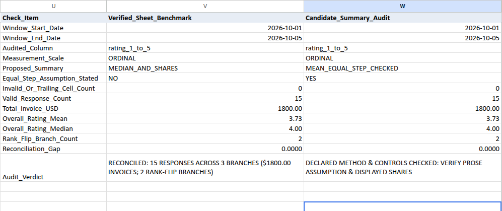
To audit a proposed chart, table, or headline summary on your own report, enter its metadata in W4:W7 and enter the candidate report’s claimed control figures in W9:W13 to compare against V9:V13 (keeping W2 = 2026-10-01, W3 = 2026-10-05, and W8 = 0 matching the verified source). In Scenarios 1 through 8 below, W9:W13 hold the same five dataset-wide baseline figures from V9:V13 (valid response count, total invoice dollars, overall rating mean, overall rating median, and rank-flip branch count) so each row isolates a scale or method choice in W4:W7, while Scenario 9 alters W9 and W11 to test a corrupted benchmark claim:
| Scenario | W4 (Audited_Column) |
W5 (Measurement_Scale) |
W6 (Proposed_Summary) |
W7 (Equal_Step) |
W9 / W10 / W11 / W12 / W13 |
W14 (Gap) |
W15 (Audit_Verdict) |
|---|---|---|---|---|---|---|---|
| Scenario 0 | NOT TESTED |
NOT TESTED |
NOT TESTED |
NOT TESTED |
All NOT TESTED |
NOT TESTED |
NOT TESTED: ENTER CANDIDATE SUMMARY AUDIT |
| Scenario 1 | postal_district |
RATIO |
MEAN_UNCONDITIONAL |
NO |
15 / 1800.00 / 3.73 / 4.00 / 2 | 0.0000 |
STOP: WRONG MEASUREMENT SCALE (postal_district IS NOMINAL, NOT RATIO) |
| Scenario 2 | outcome_code |
NOMINAL |
MEAN_UNCONDITIONAL |
NO |
15 / 1800.00 / 3.73 / 4.00 / 2 | 0.0000 |
STOP: ILLEGITIMATE SUMMARY FOR NOMINAL SCALE (NO ORDER OR EQUAL STEPS; USE MODE/COUNTS) |
| Scenario 3 | rating_1_to_5 |
ORDINAL |
MEAN_UNCONDITIONAL |
NO |
15 / 1800.00 / 3.73 / 4.00 / 2 | 0.0000 |
STOP: UNCONDITIONAL ORDINAL MEAN (STATE EQUAL-STEP ASSUMPTION & PAIR MEDIAN/SHARES) |
| Scenario 4 | rating_1_to_5 |
ORDINAL |
MEAN_EQUAL_STEP_CHECKED |
NO |
15 / 1800.00 / 3.73 / 4.00 / 2 | 0.0000 |
STOP: ORDINAL MEAN REQUIRES EXPLICIT EQUAL-STEP ASSUMPTION (SET W7=YES) |
| Scenario 5 | rating_1_to_5 |
ORDINAL |
MEAN_EQUAL_STEP_CHECKED |
YES |
15 / 1800.00 / 3.73 / 4.00 / 2 | 0.0000 |
DECLARED METHOD & CONTROLS CHECKED: VERIFY PROSE ASSUMPTION & DISPLAYED SHARES |
| Scenario 6 | rating_1_to_5 |
ORDINAL |
MEDIAN_AND_SHARES |
NO |
15 / 1800.00 / 3.73 / 4.00 / 2 | 0.0000 |
RECONCILED: DECLARED ORDINAL METHOD & BENCHMARK CONTROLS MATCH (VERIFY REPORT OUTPUT) |
| Scenario 7 | invoice_usd |
RATIO |
MEAN_UNCONDITIONAL |
NO |
15 / 1800.00 / 3.73 / 4.00 / 2 | 0.0000 |
RECONCILED: DECLARED RATIO METHOD & BENCHMARK CONTROLS MATCH (VERIFY REPORT OUTPUT) |
| Scenario 8 | response_date |
INTERVAL |
SUM_TOTAL |
NO |
15 / 1800.00 / 3.73 / 4.00 / 2 | 0.0000 |
STOP: ILLEGITIMATE SUMMARY FOR INTERVAL SCALE (SUM REQUIRES TRUE ZERO; USE MIN/MAX SPAN) |
| Scenario 9 | rating_1_to_5 |
ORDINAL |
MEDIAN_AND_SHARES |
NO |
17 / 1800.00 / 3.29 / 4.00 / 2 | 2.4400 |
STOP: SUPPORTING BENCHMARK MISMATCH (CHECK COUNTS, RATINGS, OR RANK FLIPS) |
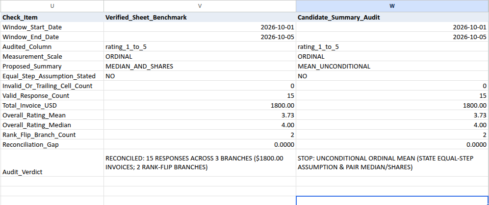
Notice the hard boundary on W14:W15: these formulas verify source health, populated-branch coverage, rollup math, scale classification (W5), declared summary method (W6), the W7 (YES/NO) flag, and the five supporting benchmark controls (W9:W13). They cannot inspect narrative slides to prove that the reader’s prose actually states the equal-step assumption, displays Bottom-2-Box / Top-2-Box share tiles, or quotes the right modal outcome label, date span, or dollar average. That is why Scenario 5 returns "DECLARED METHOD & CONTROLS CHECKED: VERIFY PROSE ASSUMPTION & DISPLAYED SHARES" and Scenarios 6 and 7 instruct you to verify the report output manually.
Step 4: Test Five Real-World Failure and Boundary Modes (and Reset Cleanly)
Run these five checks on a copy of Feedback (or restore each cell immediately) to verify that the guards stop bad reporting without silent failures:
- Text-date trap (
'2026-10-01inC2) and Google Sheets re-parsing difference: Type'2026-10-01with a leading apostrophe intoC2, then enter=ISNUMBER(C2)in a temporary scratch cell outsideA:Gsuch asY2(FALSE).H2switches to"CHECK ROW",I2:I16blank out,L2:S5display"CHECK INPUTS",V8becomes 1,V15stops with"STOP: CHECK SOURCE OR TRAILING ROWS", andW15stops with"STOP: INVALID, BLANK, OR TRAILING SOURCE ROWS". In Google Sheets (en_US), applyingFormat > Number > Datedirectly onC2automatically re-parses the text string into numeric10/1/2026(H2 = "OK"), whereas Excel for the web keeps'2026-10-01as text until you re-enter a true date or convert it. ResetC2to=DATE(2026,10,1)formattedyyyy-mm-dd, clearY2, and confirmV8 = 0andV15returns"RECONCILED: 15 RESPONSES ACROSS 3 BRANCHES ($1800.00 INVOICES; 2 RANK-FLIP BRANCHES)". - Duplicate ID (
A3 = "RSP-01") and zero rating (F3 = 0): ChangeA3alone toRSP-01(H2:H16stay"OK", whileI2andI3both change to 2; if you also changedA16toRSP-01at the same time, the count would be 3).L2:S5,V13,V14, andW14return"CHECK INPUTS", and bothV15andW15return"STOP: DUPLICATE RESPONSE IDS IN SOURCE". RestoreA3 = "RSP-02". Next, changeF3to 0 (simulating a missed score entered as zero):H3shows"CHECK ROW",V8becomes 1, andV15andW15stop. RestoreF3 = 1and confirm baseline reconciliation returns. - Stray trailing row (
A17 = "RSP-16"): TypeRSP-16intoA17without resizing the formulas.V8increments to 1 via the whole-columnCOUNTA($A:$G)check, turningV9andL2:S5to"CHECK INPUTS"and stopping bothV15andW15. ClearA17and confirmV8 = 0. - Empty branch coverage stop (
B2:B6 = "South"): Enter Scenario 5 values intoW4:W13(W4 = rating_1_to_5,W5 = ORDINAL,W6 = MEAN_EQUAL_STEP_CHECKED,W7 = YES,W8 = 0,W9 = 15,W10 = 1800.00,W11 = 3.73,W12 = 4.00), changeB2:B6toSouthsoNorthhas zero rows, and setW13 = 0(to test whether an empty-branch sheet can pass as zero rank flips). Live spreadsheet inspection confirms that not every cell inM2:S5turns to text errors:NorthdisplaysL2 = 0andM2:S2 = "CHECK INPUTS", populatedSouth(L3 = 10,M3 = 0.2000,N3 = 0.5000,O3 = 3.30,P3 = 3.50),West, andAll_Branches(O5 = 3.73from 56 ÷ 15,P5 = 4.00) keep numeric descriptive values, while all comparative ranks and guidance (Q2:S5) plusV13,V14, andW14show"CHECK INPUTS", and bothV15andW15return"STOP: EMPTY OR INCOMPLETE BRANCH COVERAGE". RestoreB2:B6toNorthand resetW4:W7,W9:W13toNOT TESTEDsoV15andW15return to baseline. - Genuine zero-flip branch alignment (
F2:F6 = 2, 2, 2, 3, 1): Keep all three branches populated and setF2:F6to2, 2, 2, 3, 1(North mean 2.00, median 2.00; overall mean 3.33, median 3.00), then enter Scenario 5’s equal-step metadata inW4:W13(W4 = rating_1_to_5,W5 = ORDINAL,W6 = MEAN_EQUAL_STEP_CHECKED,W7 = YES,W8 = 0,W9 = 15,W10 = 1800.00,W11 = 3.33,W12 = 3.00,W13 = 0). NowS5displays"BRANCH RANKS ALIGNED",V13 = 0,V15reconciles with0 RANK-FLIP BRANCHES,W14displays 0.0000, andW15returns"DECLARED METHOD & CONTROLS CHECKED: VERIFY PROSE ASSUMPTION & DISPLAYED SHARES". RestoreF2:F6to5, 1, 4, 5, 1andW4:W7,W9:W13toNOT TESTED, confirmingV15returns to"RECONCILED: 15 RESPONSES ACROSS 3 BRANCHES ($1800.00 INVOICES; 2 RANK-FLIP BRANCHES)"andW15returns to"NOT TESTED: ENTER CANDIDATE SUMMARY AUDIT".

Step 5: Resize Safely From a Fresh 15-Row Baseline Copy
This procedure resizes only the response row count while keeping the three-branch table (K2:K4 and All_Branches in K5) unchanged. Always start each new three-branch export of N responses (N >= 3, with at least one response for each listed branch, ending at row R = N + 1) from an untouched master copy of the 15-row baseline Feedback sheet (A1:W16):
- On a fresh copy of the 15-row baseline, paste your
Nresponses intoA2:G<R>(formatted consistently as numeric dates and numbers) mapped to three distinct space-free branch names matchingK2:K4. Do not delete or insert entire worksheet rows acrossK:W. - Select
H2:W16(covering all 74 baseline formula cells across rows 2 to 16) and open the Find and Replace option. In Google Sheets (Edit > Find and replace), check Also search within formulas (leaving it unchecked matches 0 formula references). In Excel for the web (Home > Find & Select > Replace), formulas update directly without a separate formula checkbox. - Replace only the six column-qualified source end tokens in
H2:W16: replace:$A$16(36 baseline sheet occurrences),:$B$16(36),:$F$16(43),:$G$16(3),:$H$16(16), and:$I$16(11) with:$A$<R>,:$B$<R>,:$F$<R>,:$G$<R>,:$H$<R>, and:$I$<R>(145 total formula-cell occurrences across the 15-row baselineH2:W16; columnsC,D, andEhave zero row-16 end bounds, and even shrinking to 9 rows at row 10 updates:$A$10through:$I$10without touching$V$10or$U$15). Never replace a bare 16 or 10. - If
N > 15, fillH2:I2down throughH<R>:I<R>. If3 <= N < 15, clear the unused baseline cellsA<R+1>:I16after step 3 (because you started from a fresh 15-row baseline copy, no prior rows exist below row 16).
What to Say in the Room
In a stakeholder review, technical scale names sound defensive. Translate the distribution directly into what changed and what action comes next:
- Don’t say: “Ordinal rating means fail strict interval assumptions across Likert scales, and
Northdrops from Rank 2 to Rank 3 on an uncalibrated parametric mean whileoutcome_codeis nominal.” - Do say: “Each branch only has 5 responses in this batch, so treat these numbers as leads to check rather than a branch ranking. West leads on both average (4.60) and middle score (5.00), with 100% of its responses at 4 or 5. North averages lower than South (3.20 vs. 3.40) because two 1-star responses pull its mean down, even though North’s middle score is 4.00 and 60% of North’s responses are 4 or 5. Those two 1-star rows were both cancelled backorders at $0.00 billed, so the first follow-up is checking parts availability at North and inspecting the notes behind South’s 60% 3-star responses.”
Frequently Asked Questions
Can you average branch rating averages when branches have different response counts?
No. If you report an overall rating average alongside the equal-step assumption, average the raw responses column (F2:F16 via O5) or compute a count-weighted average using =SUMPRODUCT(L2:L4, O2:O4)/L5. An unweighted average of branch averages gives a 5-response branch the same weight as a 150-response branch.
Why show both 1-to-2 and 4-to-5 shares instead of subtracting low scores from high scores?
A single net score collapses distinct customer experiences into identical numbers. For example, 40% top-box minus 20% bottom-box nets to +20 percentage points, and 20% top-box minus 0% bottom-box also nets to +20 percentage points, hiding the 20% dissatisfied pocket that needs operational attention.
Does switching from a 1-to-5 scale to a 1-to-7 or 1-to-10 scale make the average exact?
Wider integer scales can offer finer separation, though they do not guarantee fewer median ties in every dataset, and the numbers remain ordered categories unless step distances are formally calibrated. Conceptually, the same reporting rule applies on 1-to-7 or 1-to-10 forms: state the equal-step assumption upfront, and pair any rating average with the median and low/high score shares. Note that this workbook’s formulas (H2 validation and P2‘s cumulative median) only support integer 1-to-5 ratings, so applying the sheet to a 1-to-7 or 1-to-10 scale requires adapting and retesting the model.
Copy-Paste Formula Reference
Enter all static headers, dates, and control values from Step 1 first, then paste these 30 exact formulas into the Feedback worksheet (all quotes use standard straight ASCII quotation marks):
H2, Row validation guard (enter in H2, fill down H2:H16):
=IF(OR(COUNTA(A2:G2)<7, NOT(ISTEXT(A2)), NOT(ISTEXT(B2)), NOT(ISNUMBER(C2)), NOT(ISNUMBER(D2)), NOT(ISNUMBER(E2)), NOT(ISNUMBER(F2)), NOT(ISNUMBER(G2)), NOT(ISNUMBER($V$2)), NOT(ISNUMBER($V$3))), "CHECK ROW", IF(OR(TRIM(SUBSTITUTE(A2, CHAR(160), " "))="", TRIM(SUBSTITUTE(B2, CHAR(160), " "))="", NOT(EXACT(A2, TRIM(SUBSTITUTE(A2, CHAR(160), " ")))), NOT(EXACT(B2, TRIM(SUBSTITUTE(B2, CHAR(160), " ")))), NOT(ISERROR(FIND(" ", A2&B2))), NOT(ISERROR(FIND(CHAR(10), A2&B2))), NOT(ISERROR(FIND(CHAR(13), A2&B2))), NOT(ISERROR(FIND("*", A2&B2))), NOT(ISERROR(FIND("?", A2&B2))), NOT(ISERROR(FIND("~", A2&B2))), NOT(ISERROR(FIND("=", A2&B2))), NOT(ISERROR(FIND("<", A2&B2))), NOT(ISERROR(FIND(">", A2&B2))), LEN(A2)<6, LEN(A2)>7, NOT(EXACT(LEFT(A2, 4), "RSP-")), NOT(ISNUMBER(FIND(MID(A2, 5, 1), "0123456789"))), NOT(ISNUMBER(FIND(MID(A2, 6, 1), "0123456789"))), IF(LEN(A2)=7, NOT(ISNUMBER(FIND(MID(A2, 7, 1), "0123456789"))), FALSE), SUMPRODUCT(--EXACT($K$2:$K$4, B2))<>1, INT($V$2)<>$V$2, INT($V$3)<>$V$3, $V$2<DATE(2000,1,1), $V$3>DATE(2100,1,1), $V$3<$V$2, INT(C2)<>C2, C2<$V$2, C2>$V$3, INT(D2)<>D2, D2<100, D2>99999, INT(E2)<>E2, E2<1, E2>4, INT(F2)<>F2, F2<1, F2>5, G2<0, ROUND(G2, 2)<>G2), "CHECK ROW", "OK"))
I2, Case-sensitive response ID duplicate check (enter in I2, fill down I2:I16):
=IF(OR(NOT(EXACT(H2, "OK")), COUNTIF($H$2:$H$16, "OK")<ROWS($A$2:$A$16)), "", SUMPRODUCT(--EXACT($A$2:$A$16, A2)))
L2, Branch response count (enter in L2, fill down L2:L4):
=IF(OR($V$8>0, COUNT($I$2:$I$16)<ROWS($A$2:$A$16), COUNTIF($I$2:$I$16, ">1")>0, NOT(ISTEXT(K2)), TRIM(SUBSTITUTE(K2, CHAR(160), " "))="", NOT(EXACT(K2, TRIM(SUBSTITUTE(K2, CHAR(160), " ")))), SUMPRODUCT(--EXACT($K$2:$K$4, K2))<>1), "CHECK INPUTS", SUMPRODUCT(--EXACT($B$2:$B$16, K2)))
M2, Branch Bottom-2-Box share, ratings 1 and 2 (enter in M2, fill down M2:M4; keep unrounded, format as 0.0000 or 0.00%):
=IF(OR(NOT(ISNUMBER(L2)), L2<=0), "CHECK INPUTS", SUMPRODUCT(--EXACT($B$2:$B$16, K2), --($F$2:$F$16<=2))/L2)
N2, Branch Top-2-Box share, ratings 4 and 5 (enter in N2, fill down N2:N4; keep unrounded, format as 0.0000 or 0.00%):
=IF(OR(NOT(ISNUMBER(L2)), L2<=0), "CHECK INPUTS", SUMPRODUCT(--EXACT($B$2:$B$16, K2), --($F$2:$F$16>=4))/L2)
O2, Branch rating mean (enter in O2, fill down O2:O4; keep unrounded, format as 0.00):
=IF(OR(NOT(ISNUMBER(L2)), L2<=0), "CHECK INPUTS", SUMPRODUCT(--EXACT($B$2:$B$16, K2), $F$2:$F$16)/L2)
P2, Branch rating median over integers 1 to 5 (enter in P2, fill down P2:P4; keep unrounded, format as 0.00):
=IF(OR(NOT(ISNUMBER(L2)), L2<=0), "CHECK INPUTS", (1+IF(INT((L2+1)/2)>SUMPRODUCT(--EXACT($B$2:$B$16, K2), --($F$2:$F$16<=1)), 1, 0)+IF(INT((L2+1)/2)>SUMPRODUCT(--EXACT($B$2:$B$16, K2), --($F$2:$F$16<=2)), 1, 0)+IF(INT((L2+1)/2)>SUMPRODUCT(--EXACT($B$2:$B$16, K2), --($F$2:$F$16<=3)), 1, 0)+IF(INT((L2+1)/2)>SUMPRODUCT(--EXACT($B$2:$B$16, K2), --($F$2:$F$16<=4)), 1, 0)+1+IF(INT((L2+2)/2)>SUMPRODUCT(--EXACT($B$2:$B$16, K2), --($F$2:$F$16<=1)), 1, 0)+IF(INT((L2+2)/2)>SUMPRODUCT(--EXACT($B$2:$B$16, K2), --($F$2:$F$16<=2)), 1, 0)+IF(INT((L2+2)/2)>SUMPRODUCT(--EXACT($B$2:$B$16, K2), --($F$2:$F$16<=3)), 1, 0)+IF(INT((L2+2)/2)>SUMPRODUCT(--EXACT($B$2:$B$16, K2), --($F$2:$F$16<=4)), 1, 0))/2)
Q2, Full-precision branch mean competition rank (enter in Q2, fill down Q2:Q4):
=IF(OR(NOT(ISNUMBER(O2)), COUNT($O$2:$O$4)<ROWS($K$2:$K$4)), "CHECK INPUTS", 1+SUMPRODUCT(--($O$2:$O$4>O2)))
R2, Full-precision branch median competition rank (enter in R2, fill down R2:R4):
=IF(OR(NOT(ISNUMBER(P2)), COUNT($P$2:$P$4)<ROWS($K$2:$K$4)), "CHECK INPUTS", 1+SUMPRODUCT(--($P$2:$P$4>P2)))
S2, Branch scale guidance flag (enter in S2, fill down S2:S4):
=IF(OR(NOT(ISNUMBER(Q2)), NOT(ISNUMBER(R2)), NOT(ISNUMBER(M2)), NOT(ISNUMBER(N2))), "CHECK INPUTS", IF(Q2<>R2, "RANK FLIP: REPORT MEDIAN & SHARES", IF(AND(M2>0, N2>0), "POLARIZED: PAIR MEAN WITH SHARES", "ALIGNED: MEAN OK IF EQUAL-STEP STATED")))
L5, All_Branches response count rollup (enter in L5):
=IF(OR(NOT(EXACT(K5, "All_Branches")), COUNT($L$2:$L$4)<ROWS($K$2:$K$4)), "CHECK INPUTS", SUM($L$2:$L$4))
M5, All_Branches Bottom-2-Box share (enter in M5; keep unrounded, format as 0.0000 or 0.00%):
=IF(OR(NOT(ISNUMBER(L5)), L5<=0), "CHECK INPUTS", COUNTIF($F$2:$F$16, "<=2")/L5)
N5, All_Branches Top-2-Box share (enter in N5; keep unrounded, format as 0.0000 or 0.00%):
=IF(OR(NOT(ISNUMBER(L5)), L5<=0), "CHECK INPUTS", COUNTIF($F$2:$F$16, ">=4")/L5)
O5, All_Branches overall rating mean (enter in O5; keep unrounded, format as 0.00):
=IF(OR(NOT(ISNUMBER(L5)), L5<=0), "CHECK INPUTS", AVERAGE($F$2:$F$16))
P5, All_Branches overall rating median (enter in P5; keep unrounded, format as 0.00):
=IF(OR(NOT(ISNUMBER(L5)), L5<=0), "CHECK INPUTS", MEDIAN($F$2:$F$16))
Q5, All_Branches mean rank guard (enter in Q5):
=IF(COUNT($Q$2:$Q$4)<ROWS($K$2:$K$4), "CHECK INPUTS", "ALL BRANCHES")
R5, All_Branches median rank guard (enter in R5):
=IF(COUNT($R$2:$R$4)<ROWS($K$2:$K$4), "CHECK INPUTS", "ALL BRANCHES")
S5, All_Branches overall rank-flip summary (enter in S5):
=IF(OR(NOT(ISNUMBER(L5)), COUNT($Q$2:$Q$4)<ROWS($K$2:$K$4), COUNT($R$2:$R$4)<ROWS($K$2:$K$4)), "CHECK INPUTS", IF(COUNTIF($S$2:$S$4, "RANK FLIP*")>0, "BRANCH RANK FLIP PRESENT (" & COUNTIF($S$2:$S$4, "RANK FLIP*") & " OF " & ROWS($K$2:$K$4) & ")", "BRANCH RANKS ALIGNED"))
V5, Active audited column scale lookup (enter in V5):
=IF(NOT(ISTEXT(IF(EXACT(W4, "NOT TESTED"), V4, W4))), "UNKNOWN COLUMN", IF(OR(EXACT(IF(EXACT(W4, "NOT TESTED"), V4, W4), "response_id"), EXACT(IF(EXACT(W4, "NOT TESTED"), V4, W4), "branch"), EXACT(IF(EXACT(W4, "NOT TESTED"), V4, W4), "postal_district"), EXACT(IF(EXACT(W4, "NOT TESTED"), V4, W4), "outcome_code")), "NOMINAL", IF(EXACT(IF(EXACT(W4, "NOT TESTED"), V4, W4), "response_date"), "INTERVAL", IF(EXACT(IF(EXACT(W4, "NOT TESTED"), V4, W4), "rating_1_to_5"), "ORDINAL", IF(EXACT(IF(EXACT(W4, "NOT TESTED"), V4, W4), "invoice_usd"), "RATIO", "UNKNOWN COLUMN")))))
V6, Default legitimate summary method lookup (enter in V6):
=IF(EXACT(V5, "NOMINAL"), "MODE_AND_COUNTS", IF(EXACT(V5, "INTERVAL"), "MIN_MAX_SPAN", IF(EXACT(V5, "ORDINAL"), "MEDIAN_AND_SHARES", IF(EXACT(V5, "RATIO"), "MEAN_UNCONDITIONAL", "CHECK COLUMN"))))
V8, Invalid, blank, and whole-column trailing cell counter across A:G (enter in V8):
=COUNTIF($H$2:$H$16, "<>OK")+COUNTBLANK($A$2:$G$16)+(COUNTA($A:$G)-COUNTA($A$1:$G$16))
V9, Verified valid response count benchmark (enter in V9):
=IF(OR(V8>0, COUNT($I$2:$I$16)<ROWS($A$2:$A$16)), "CHECK INPUTS", COUNTA($A$2:$A$16))
V10, Verified total invoice USD benchmark (enter in V10):
=IF(NOT(ISNUMBER(V9)), "CHECK INPUTS", ROUND(SUM($G$2:$G$16), 2))
V11, Rounded 2-decimal overall rating mean control for W11 checks (enter in V11):
=IF(OR(NOT(ISNUMBER(V9)), NOT(ISNUMBER(O5))), "CHECK INPUTS", ROUND(O5, 2))
V12, Rounded 2-decimal overall rating median control for W12 checks (enter in V12):
=IF(OR(NOT(ISNUMBER(V9)), NOT(ISNUMBER(P5))), "CHECK INPUTS", ROUND(P5, 2))
V13, Verified rank-flip branch count benchmark (enter in V13):
=IF(OR(NOT(ISNUMBER(V9)), NOT(ISNUMBER(L5)), COUNT($L$2:$L$4)<ROWS($K$2:$K$4), COUNTIF($L$2:$L$4, "<=0")>0, COUNT($M$2:$M$4)<ROWS($K$2:$K$4), COUNT($N$2:$N$4)<ROWS($K$2:$K$4), COUNT($O$2:$O$4)<ROWS($K$2:$K$4), COUNT($P$2:$P$4)<ROWS($K$2:$K$4), COUNT($Q$2:$Q$4)<ROWS($K$2:$K$4), COUNT($R$2:$R$4)<ROWS($K$2:$K$4), (COUNTIF($S$2:$S$4, "RANK FLIP*")+COUNTIF($S$2:$S$4, "POLARIZED:*")+COUNTIF($S$2:$S$4, "ALIGNED:*"))<ROWS($K$2:$K$4), IF(ISTEXT(Q5), NOT(EXACT(Q5, "ALL BRANCHES")), TRUE), IF(ISTEXT(R5), NOT(EXACT(R5, "ALL BRANCHES")), TRUE), IF(ISTEXT(S5), EXACT(S5, "CHECK INPUTS"), TRUE)), "CHECK INPUTS", COUNTIF($S$2:$S$4, "RANK FLIP*"))
V14, Exact integer-count and sum reconciliation gap between L2:O5 and source rows (enter in V14):
=IF(OR(NOT(ISNUMBER(V9)), NOT(ISNUMBER(L5)), NOT(ISNUMBER(M5)), NOT(ISNUMBER(N5)), NOT(ISNUMBER(O5)), NOT(ISNUMBER(V10)), NOT(ISNUMBER(V11)), NOT(ISNUMBER(V12)), NOT(ISNUMBER(V13)), COUNT($L$2:$L$4)<ROWS($K$2:$K$4), COUNTIF($L$2:$L$4, "<=0")>0, COUNT($M$2:$M$4)<ROWS($K$2:$K$4), COUNT($N$2:$N$4)<ROWS($K$2:$K$4), COUNT($O$2:$O$4)<ROWS($K$2:$K$4), COUNT($P$2:$P$4)<ROWS($K$2:$K$4)), "CHECK INPUTS", ROUND(ABS(L5-V9)+ABS(V9-ROWS($A$2:$A$16))+COUNTIF($I$2:$I$16, ">1")+ABS(ROUND(SUMPRODUCT($L$2:$L$4, $M$2:$M$4)-COUNTIF($F$2:$F$16, "<=2"), 8))+ABS(ROUND(SUMPRODUCT($L$2:$L$4, $N$2:$N$4)-COUNTIF($F$2:$F$16, ">=4"), 8))+ABS(ROUND(SUMPRODUCT($L$2:$L$4, $O$2:$O$4)-SUM($F$2:$F$16), 8))+ABS(ROUND(L5*M5-COUNTIF($F$2:$F$16, "<=2"), 8))+ABS(ROUND(L5*N5-COUNTIF($F$2:$F$16, ">=4"), 8))+ABS(ROUND(L5*O5-SUM($F$2:$F$16), 8)), 4))
V15, Verified source benchmark audit verdict (enter in V15):
=IF(OR(V8>0, NOT(ISNUMBER(V9))), "STOP: CHECK SOURCE OR TRAILING ROWS", IF(COUNTIF($I$2:$I$16, ">1")>0, "STOP: DUPLICATE RESPONSE IDS IN SOURCE", IF(OR(COUNT($L$2:$L$4)<ROWS($K$2:$K$4), COUNTIF($L$2:$L$4, "<=0")>0, NOT(ISNUMBER(V13))), "STOP: EMPTY OR INCOMPLETE BRANCH COVERAGE", IF(IF(ISNUMBER(V14), V14<>0, TRUE), "STOP: BRANCH ROLLUP RECONCILIATION GAP", "RECONCILED: " & V9 & " RESPONSES ACROSS " & ROWS($K$2:$K$4) & " BRANCHES ($" & TEXT(V10, "0.00") & " INVOICES; " & V13 & " RANK-FLIP BRANCHES)"))))
W14, Candidate summary vs. verified benchmark control gap (enter in W14):
=IF(OR(V8>0, NOT(ISNUMBER(V9)), COUNT($L$2:$L$4)<ROWS($K$2:$K$4), COUNTIF($L$2:$L$4, "<=0")>0, NOT(ISNUMBER(V13)), NOT(ISNUMBER(V14)), COUNTIF($I$2:$I$16, ">1")>0, IF(ISNUMBER(V14), V14<>0, TRUE), NOT(ISNUMBER(V10)), NOT(ISNUMBER(V11)), NOT(ISNUMBER(V12)), NOT(ISNUMBER(W2)), NOT(ISNUMBER(W3)), NOT(ISNUMBER(W8))), "CHECK INPUTS", IF(OR(INT(W2)<>W2, INT(W3)<>W3, W2<>V2, W3<>V3, INT(W8)<>W8, W8<>0), "CHECK INPUTS", IF(IF(AND(ISTEXT(W4), ISTEXT(W5), ISTEXT(W6), ISTEXT(W7), ISTEXT(W9), ISTEXT(W10), ISTEXT(W11), ISTEXT(W12), ISTEXT(W13)), AND(EXACT(W4, "NOT TESTED"), EXACT(W5, "NOT TESTED"), EXACT(W6, "NOT TESTED"), EXACT(W7, "NOT TESTED"), EXACT(W9, "NOT TESTED"), EXACT(W10, "NOT TESTED"), EXACT(W11, "NOT TESTED"), EXACT(W12, "NOT TESTED"), EXACT(W13, "NOT TESTED")), FALSE), "NOT TESTED", IF(OR(NOT(ISTEXT(W4)), NOT(ISTEXT(W5)), NOT(ISTEXT(W6)), NOT(ISTEXT(W7)), NOT(ISNUMBER(W9)), NOT(ISNUMBER(W10)), NOT(ISNUMBER(W11)), NOT(ISNUMBER(W12)), NOT(ISNUMBER(W13))), "CHECK INPUTS", IF(OR(INT(W9)<>W9, W9<=0, W10<0, ROUND(W10, 2)<>W10, W11<1, W11>5, ROUND(W11, 2)<>W11, W12<1, W12>5, ROUND(W12, 2)<>W12, INT(W13)<>W13, W13<0), "CHECK INPUTS", ROUND(ABS(W9-V9)+ABS(W10-V10)+ABS(W11-V11)+ABS(W12-V12)+ABS(W13-V13), 4))))))
W15, Candidate measurement scale and method audit verdict (enter in W15):
=IF(OR(V8>0, NOT(ISNUMBER(V9))), "STOP: INVALID, BLANK, OR TRAILING SOURCE ROWS", IF(COUNTIF($I$2:$I$16, ">1")>0, "STOP: DUPLICATE RESPONSE IDS IN SOURCE", IF(OR(COUNT($L$2:$L$4)<ROWS($K$2:$K$4), COUNTIF($L$2:$L$4, "<=0")>0, NOT(ISNUMBER(V13))), "STOP: EMPTY OR INCOMPLETE BRANCH COVERAGE", IF(IF(ISNUMBER(V14), V14<>0, TRUE), "STOP: BRANCH ROLLUP RECONCILIATION GAP", IF(IF(AND(ISNUMBER(W2), ISNUMBER(W3)), OR(INT(W2)<>W2, INT(W3)<>W3, W2<>V2, W3<>V3), TRUE), "STOP: EXTRACT WINDOW MISMATCH", IF(IF(ISNUMBER(W8), OR(INT(W8)<>W8, W8<>0), TRUE), "STOP: INVALID CLAIM ROW-CHECK COUNT", IF(EXACT(W14, "NOT TESTED"), "NOT TESTED: ENTER CANDIDATE SUMMARY AUDIT", IF(OR(EXACT(W14, "CHECK INPUTS"), NOT(OR(EXACT(W7, "YES"), EXACT(W7, "NO")))), "STOP: INVALID OR INCOMPLETE CANDIDATE INPUTS", IF(EXACT(V5, "UNKNOWN COLUMN"), "STOP: UNKNOWN AUDITED COLUMN", IF(NOT(OR(EXACT(W5, "NOMINAL"), EXACT(W5, "ORDINAL"), EXACT(W5, "INTERVAL"), EXACT(W5, "RATIO"))), "STOP: UNKNOWN MEASUREMENT SCALE", IF(NOT(EXACT(W5, V5)), "STOP: WRONG MEASUREMENT SCALE (" & W4 & " IS " & V5 & ", NOT " & W5 & ")", IF(NOT(OR(EXACT(W6, "MODE_AND_COUNTS"), EXACT(W6, "MIN_MAX_SPAN"), EXACT(W6, "MEDIAN_AND_SHARES"), EXACT(W6, "MEAN_EQUAL_STEP_CHECKED"), EXACT(W6, "MEAN_UNCONDITIONAL"), EXACT(W6, "SUM_TOTAL"))), "STOP: UNKNOWN SUMMARY METHOD", IF(W14<>0, "STOP: SUPPORTING BENCHMARK MISMATCH (CHECK COUNTS, RATINGS, OR RANK FLIPS)", IF(EXACT(W5, "NOMINAL"), IF(NOT(EXACT(W6, "MODE_AND_COUNTS")), "STOP: ILLEGITIMATE SUMMARY FOR NOMINAL SCALE (NO ORDER OR EQUAL STEPS; USE MODE/COUNTS)", IF(EXACT(W7, "YES"), "STOP: EQUAL-STEP ASSUMPTION DOES NOT APPLY TO MODE/COUNTS", "RECONCILED: DECLARED " & W5 & " METHOD & BENCHMARK CONTROLS MATCH (VERIFY REPORT OUTPUT)")), IF(EXACT(W5, "INTERVAL"), IF(EXACT(W6, "SUM_TOTAL"), "STOP: ILLEGITIMATE SUMMARY FOR INTERVAL SCALE (SUM REQUIRES TRUE ZERO; USE MIN/MAX SPAN)", IF(NOT(OR(EXACT(W6, "MIN_MAX_SPAN"), EXACT(W6, "MEAN_UNCONDITIONAL"))), "STOP: UNSUPPORTED SUMMARY FOR INTERVAL SCALE", IF(EXACT(W7, "YES"), "STOP: EQUAL-STEP ASSUMPTION DOES NOT APPLY TO INTERVAL SCALE", "RECONCILED: DECLARED " & W5 & " METHOD & BENCHMARK CONTROLS MATCH (VERIFY REPORT OUTPUT)"))), IF(EXACT(W5, "ORDINAL"), IF(EXACT(W6, "MEAN_UNCONDITIONAL"), "STOP: UNCONDITIONAL ORDINAL MEAN (STATE EQUAL-STEP ASSUMPTION & PAIR MEDIAN/SHARES)", IF(EXACT(W6, "MEAN_EQUAL_STEP_CHECKED"), IF(EXACT(W7, "YES"), "DECLARED METHOD & CONTROLS CHECKED: VERIFY PROSE ASSUMPTION & DISPLAYED SHARES", "STOP: ORDINAL MEAN REQUIRES EXPLICIT EQUAL-STEP ASSUMPTION (SET W7=YES)"), IF(OR(EXACT(W6, "MEDIAN_AND_SHARES"), EXACT(W6, "MODE_AND_COUNTS")), IF(EXACT(W7, "YES"), "STOP: EQUAL-STEP ASSUMPTION APPLIES ONLY TO ORDINAL MEAN", "RECONCILED: DECLARED " & W5 & " METHOD & BENCHMARK CONTROLS MATCH (VERIFY REPORT OUTPUT)"), "STOP: ILLEGITIMATE SUMMARY FOR ORDINAL SCALE (USE MEDIAN & SHARES OR ASSUMPTION-CHECKED MEAN)"))), IF(NOT(OR(EXACT(W6, "MEAN_UNCONDITIONAL"), EXACT(W6, "SUM_TOTAL"), EXACT(W6, "MEDIAN_AND_SHARES"), EXACT(W6, "MIN_MAX_SPAN"))), "STOP: UNSUPPORTED SUMMARY FOR RATIO SCALE", IF(EXACT(W7, "YES"), "STOP: UNNECESSARY EQUAL-STEP ASSUMPTION FLAG FOR RATIO SCALE", "RECONCILED: DECLARED " & W5 & " METHOD & BENCHMARK CONTROLS MATCH (VERIFY REPORT OUTPUT)"))))))))))))))))))