
To save a month-end spreadsheet snapshot without breaking formulas, leave the live summary alone. First type the close month, a fixed close date, and the control total from your accounting system. Then copy the closed month’s summary into a separate range with Paste values only: Ctrl+Shift+V in Google Sheets, or Values only from the Paste menu in Excel for the web. Check that no formulas remain there, and protect it.
In the April example below, the live summary shows $12,000.00 across 8 orders. A week after close, a late credit lowers one order by $800.00. If the snapshot was pasted with a regular paste, it quietly rewrites itself to $12,000.00 − $800.00 = $11,200.00. If it was pasted as values, it stays at $12,000.00, and the sheet flags the −$800.00 change so you can decide what to do about it.
My preferred tool is Google Sheets because a spreadsheet should be shareable. It should make collaborating with others easy. Every step below also covers Excel for the web. The live summary here is a COUNTIFS and SUMIFS grid, the kind compared in SUMIFS or pivot table for monthly reporting. Before you freeze anything, make sure the month actually loaded into your report.
The results below come from a test of this exact workbook in Google Sheets and Excel for the web, both in US English. Desktop Excel wasn’t part of the test.
The Example Ledger
Below is the 8-order April 2026 ledger I made up for this article. It sits on a sheet named Month_Close, with headings in A1:D1 and orders in rows 2 to 9. The Row column is a row-number guide, not a worksheet column.
| Row | order_id (A) | order_date (B) | service_line (C) | net_sales_usd (D) |
|---|---|---|---|---|
| 2 | ORD-7201 | 2026-04-03 | Hardware | $1,800.00 |
| 3 | ORD-7202 | 2026-04-07 | Software | $1,500.00 |
| 4 | ORD-7203 | 2026-04-11 | Support | $1,500.00 |
| 5 | ORD-7204 | 2026-04-14 | Software | $2,000.00 |
| 6 | ORD-7205 | 2026-04-18 | Hardware | $1,500.00 |
| 7 | ORD-7206 | 2026-04-22 | Training | $1,400.00 |
| 8 | ORD-7207 | 2026-04-27 | Support | $1,100.00 |
| 9 | ORD-7208 | 2026-04-30 | Hardware | $1,200.00 |
April totals $12,000.00: Hardware is $4,500.00 across 3 orders, Software is $3,500.00 across 2, Support is $2,600.00 across 2, and Training is $1,400.00 from 1 order. The books close on 2026-05-02, and the accounting system’s close report also says $12,000.00.
Here’s what five ways of saving April do when that late $800.00 credit arrives on ORD-7204:
| Method | Live summary still calculates? | Saved April total after the credit | Close date stays fixed? | What the check block says |
|---|---|---|---|---|
| Paste values into a separate range | Yes | $12,000.00 | Yes | Alert: live April changed by −$800.00, snapshot preserved |
| Paste values over the live summary | No | $12,000.00, but the summary no longer updates | Yes | Stop: live summary formulas overwritten |
| Regular paste into a separate range | Yes | $11,200.00 | Yes | Stop: snapshot not frozen, 5 formula rows |
Values, with =TODAY() as the close date |
Yes | $12,000.00 | No | Stop: formula in the close stamp |
| Version history only | Yes | Only inside an older version of the file | File timestamp only | No check is possible inside the sheet |
Only the first row keeps the live model, the closed numbers, and the close date intact.
Why the Common Shortcuts Fail
Pasting values over the live summary. Selecting the summary and pasting it onto itself as values freezes April in place. It also deletes the formulas that made it a summary. From then on, new orders and corrections don’t change it, and nothing on the sheet says so unless you check for formulas.
A regular paste into a separate range. Copy the summary in I2:K6 and paste it into N2:P6 with Ctrl+V, and the service-line names arrive as plain text, but the counts and dollars arrive as formulas. Their ledger ranges are anchored with $ signs, such as $D$2:$D$9, so they still read the live ledger. In the test, on a disposable copy of the tab, changing ORD-7204 in D5 from $2,000.00 to $1,200.00 dropped the “snapshot” total in P6 to $11,200.00. The order count in O6 still said 8, so nothing looked wrong at a glance.
Duplicating the tab. A copy of a self-contained tab copies its own ledger too. Editing the original ledger afterward doesn’t change the copy, but now you have two ledgers, and the copy’s formulas are still live. In desktop Excel, moving or copying a sheet to another workbook can also create links back to the source file when the sheet’s formulas point at other sheets you didn’t copy. Microsoft documents that those workbook links can trigger a prompt to enable content when the file opens.
=TODAY() as the close date. TODAY() returns the current date every time the sheet recalculates, so it can’t record when you closed. In the test, a close date entered as =TODAY() showed 2026-11-18, the day of the test, not the close date. A snapshot saved on 2026-05-02 and opened on 2026-05-18 would show a close date 16 days late. Type the date instead. In Google Sheets, Ctrl+; enters today’s date as a fixed value.
Freezing too early or from a stale export. A snapshot saved on April 25 covers only the first 6 orders. It shows $9,700.00 and misses ORD-7207 and ORD-7208, so it’s $1,100.00 + $1,200.00 = $2,300.00 short. Pasting a stale 6-order export on May 2 gives the same wrong $9,700.00 with a correct-looking date. Save the snapshot only after the month ends, and compare it with the control total from your accounting or point-of-sale system.
Relying on version history alone. Version history is useful, but it doesn’t replace a frozen snapshot:
- Google Sheets: according to Google’s version history help, only people with edit access can see earlier versions. You can name up to 15 versions per spreadsheet. That limit applies to named versions, not to every saved revision. Restoring an earlier version changes the live file, and Google notes that it clears the cell-by-cell edit history from before the restore. If you need to keep that history, Google recommends making a copy of the spreadsheet instead of restoring.
- Excel: according to Microsoft’s version history help, version history needs the file stored in OneDrive or SharePoint, so a file saved only on your computer doesn’t have it. Microsoft says personal accounts can get back the last 25 versions. Work and school accounts follow their library’s settings. Restoring replaces the current workbook.
Neither one lets a formula compare April as you closed it with April as it reads today. A snapshot inside the workbook does.
Step 1: Keep the Live Ledger and Live Summary Separate
The workbook uses one sheet, Month_Close, with four blocks side by side:
A1:G9holds the ledger in columns A to D, plus helper formulas in E to G.I1:L6holds the live monthly summary.N1:S6holds the frozen snapshot and its checks.U1:W18holds the close stamp and the check block.
Leave columns H, M, and T empty as spacers. Enter dates as real dates and amounts as plain numbers (1800, not “$1,800”). Then paste the formulas from the Formula Reference at the end before you try any of the steps below. Until the close month is typed in V2, which is the first move in Step 2, the summary shows "CHECK INPUTS" instead of numbers.
The helper columns prepare each order for the summary. Column E checks the row and returns "OK" or "CHECK ROW". Column F turns the date into a month label with TEXT(B2, "yyyy-mm"), so April orders read 2026-04. Column G compares that label with the close month in V2. It marks April orders "IN CLOSED MONTH" and later orders "OTHER MONTH".
The helper formulas are strict on purpose, so the example flags a doubtful row instead of guessing. Column E marks a row "CHECK ROW", and the checks stop, unless all of these are true:
- The order ID is uppercase text with no spaces, such as ORD-7201, and appears only once. The duplicate check ignores case.
- The date is a whole date from 2000-01-01 to 2100-01-01, with no time attached.
- The amount is a number of zero or more, with no more than two decimal places.
- Neither the order ID nor the service line contains a line break or any of these characters: * ? ~ = < >
The close month in V2 must be text in the form YYYY-MM, such as 2026-04. These are rules of this example workbook, not limits of Paste values only. A credit entered as a negative row fails the check. In this example, a late credit is a correction to the original order’s amount. If your ledger records credits as separate negative rows, redesign and retest the checks first.
The live summary counts and adds the orders for the close month by service line:
| Row | service_line (I) | live_order_count (J) | live_net_sales_usd (K) | Live_Formula_Check (L) |
|---|---|---|---|---|
| 2 | Hardware | 3 | $4,500.00 | LIVE FORMULA |
| 3 | Software | 2 | $3,500.00 | LIVE FORMULA |
| 4 | Support | 2 | $2,600.00 | LIVE FORMULA |
| 5 | Training | 1 | $1,400.00 | LIVE FORMULA |
| 6 | Summary_Total | 8 | $12,000.00 | LIVE FORMULA |

At its core, J2 is COUNTIFS($F$2:$F$9, $V$2, $C$2:$C$9, $I2). The full version in the Formula Reference wraps it in input checks. K2 adds the dollars:
=IF(NOT(ISNUMBER(J2)), "CHECK INPUTS", ROUND(SUMIFS($D$2:$D$9, $F$2:$F$9, $V$2, $C$2:$C$9, $I2), 2))
ROUND(..., 2) is this workbook’s own rule. It keeps every total to whole cents, so later comparisons don’t trip over tiny decimal leftovers. Type the four service lines in I2:I5 and Summary_Total in I6. Copy J2:L2 down to row 5. Row 6 has its own total formulas.
Column L is the guard against Scenario 2 from the table above. L2 uses ISFORMULA on J2 and on K2 separately, and it returns "BROKEN: STATIC OVERWRITE" if either one holds a typed number. Check one cell at a time. Google’s ISFORMULA documentation says that on a range it checks only the first cell. In the test, a range ISFORMULA returned a single result in Google Sheets, while in Excel for the web, =ISFORMULA(Month_Close!J2:J6) spilled one result per row.
ISFORMULA only tells you that a formula is there, not that it’s the right one. In the test, K2 was replaced with =4500. Column L still said LIVE FORMULA, and the checks still reconciled, even after an April order in D2 changed to $1,900.00. If you suspect someone edited a formula, compare it with the Formula Reference.
Step 2: Freeze the Closed Month Next to the Live Summary
Once the month has closed and the control total is final, save the snapshot in N1:S6, right next to the live summary. Type the headings in N1:S1 first. They’re listed in the Formula Reference.
- Type the close stamp. Put 2026-04 in
V2as text. Typing an apostrophe first (‘2026-04) stops the spreadsheet from turning it into a date. Put the date you’re saving the snapshot, 2026-05-02 in the example, inV3as a typed date. Put 12000 from the accounting close report inV4. - Check the live summary before you copy it.
J6should show 8,K6should show $12,000.00, andL2:L6should all say LIVE FORMULA. If any of them says"CHECK INPUTS", fix that first, because freezing now would save those words instead of numbers. At this point,V18saysSTOP: INVALID OR BLANK CELLS IN FROZEN SNAPSHOT. That’s expected, because the snapshot is still empty. - Select
I2:K6and copy it. - Click
N2and paste values only. In Google Sheets, press Ctrl+Shift+V (Cmd+Shift+V on a Mac), or choose Edit > Paste special > Values only. In Excel for the web, on the Home tab, open the Paste menu and choose Values only, or press Ctrl+Shift+V. - Because
I6and the snapshot both use the label Summary_Total, one paste fills all 15 cells inN2:P6.V18should now start with RECONCILED. - Protect the saved values in
N2:P6and the close stamp inV2:V4.
The snapshot now holds plain numbers:
| Row | snapshot_service_line (N) | snapshot_order_count (O) | snapshot_net_sales_usd (P) | Snapshot_Freeze_Check (Q) | Abs_Row_Count_Drift (R) | Abs_Row_Sales_Drift_USD (S) |
|---|---|---|---|---|---|---|
| 2 | Hardware | 3 | $4,500.00 | FROZEN VALUE | 0 | $0.00 |
| 3 | Software | 2 | $3,500.00 | FROZEN VALUE | 0 | $0.00 |
| 4 | Support | 2 | $2,600.00 | FROZEN VALUE | 0 | $0.00 |
| 5 | Training | 1 | $1,400.00 | FROZEN VALUE | 0 | $0.00 |
| 6 | Summary_Total | 8 | $12,000.00 | FROZEN VALUE | 0 | $0.00 |

Columns Q to S are formulas on purpose. Copy Q2:S2 down to row 6. Only N2:P6 is the saved data. Q2 checks N2, O2, and P2 one at a time with ISFORMULA. It returns "FROZEN VALUE" when all three are plain values and "UNFROZEN FORMULA" when any of them still holds a formula. R2 and S2 compare the frozen row with the live row beside it. They show how far the live order count and dollars have moved since close, ignoring direction.
Protecting the snapshot. In Google Sheets, choose Data > Protect sheets and ranges, add N2:P6 and V2:V4, and set the permissions. Google’s protection help describes both options:
- Show a warning when editing this range doesn’t stop anyone. In the test, typing over a protected
P2showed a “Heads up!” prompt asking whether to edit anyway. Google’s documentation confirms that a warning doesn’t block the edit. - Restrict who can edit this range limits editing to the people you choose, such as Only you. Owners can still edit protected ranges.
Leave the ledger and W2:W11 outside the protected ranges, so people can keep entering orders and checking other copies.
In Excel for the web, choose Review > Manage Protection and turn on Protect sheet, as Microsoft’s worksheet protection help describes. Sheet protection covers the whole sheet, so add the cells people still need to type in under Unlocked ranges: the ledger in A2:D9, and W2:W11 if you’ll check other saved copies in Step 3. Desktop Excel uses a different menu.
The test checked these settings from the owner’s account only, so blocking another collaborator wasn’t tested. Protection also stops edits, not viewing or copying. For the details, see how to protect formula cells in a shared Google Sheet and why dashboard filters aren’t row-level access controls.
If you want the snapshot on another tab or in another file. This walkthrough works because the snapshot and the live summary sit on the same sheet. In the test, pasting only N2:S6 onto a blank tab gave "FROZEN VALUE" in column Q but "CHECK INPUTS" in columns R and S, because the live summary they compare against wasn’t there. A separate archive tab needs its own typed close stamp and formulas that point back at the live sheet, such as Month_Close!J2. This article doesn’t build that version.
For a separate archive file, freeze first and move second. Google’s Paste special works only within one spreadsheet, and a copied tab that still holds formulas can lose the sheets those formulas read. So make a values-only copy inside the source workbook, with the close month, close date, and control total typed beside the values. Then move that frozen copy to the archive file:
- Google Sheets: right-click the tab and choose Copy to > Existing spreadsheet.
- Excel for the web: Microsoft notes that the sheet tab menu can’t move or copy a sheet to another workbook. Instead, copy the frozen data and paste it into a blank sheet in the archive workbook. Desktop Excel also offers Move or Copy.
Pasting values after a broken copy doesn’t bring back the missing numbers. The transfer to a separate file wasn’t part of the test.
Step 3: Check the Snapshot and Catch Post-Close Edits
The check block in U1:W18 answers two questions. Column V asks whether the snapshot matches the live summary and the control total. Column W lets you check another saved copy, such as an archive file someone else made, against that snapshot.
| Row | Metric (U) | Column V at baseline | What goes in column W |
|---|---|---|---|
| 2 | Close_Month | 2026-04 (typed) | Close month of the other copy |
| 3 | Snapshot_Saved_Date | 2026-05-02 (typed) | Date the other copy was saved |
| 4 | Signed_Control_Total_USD | 12000.00 (typed) | Control total recorded with it |
| 5 | Invalid_Row_Or_Rule_Count | 0 | Type 0 (guard cell) |
| 6 | Trailing_Cells_Below_Tables | 0 | Type 0 (guard cell) |
| 7 | Unfrozen_Snapshot_Rows | 0 | Saved rows that still hold a formula (see below) |
| 8 | Snapshot_Order_Count | 8 | Its order count |
| 9 | Snapshot_Total_Sales_USD | 12000.00 | Its total sales |
| 10 | Snapshot_Top_Service_USD | 4500.00 | Its largest service line |
| 11 | Snapshot_Min_Service_USD | 1400.00 | Its smallest service line |
| 12 | Live_Closed_Month_Sales_USD | 12000.00 | Formula: its total minus the snapshot’s |
| 13 | Snapshot_vs_Control_Gap_USD | 0.00 | Formula: its total minus the control total |
| 14 | Snapshot_Internal_Sales_Gap_USD | 0.00 | Formula: shift in the largest and smallest lines |
| 15 | Snapshot_Internal_Count_Gap | 0 | Formula: its orders minus the snapshot’s |
| 16 | Post_Close_Net_Drift_USD | 0.00 | Formula: days between its date and the close date |
| 17 | Post_Close_Abs_Category_Drift_USD | 0.00 | Formula: the W7 count, once the inputs pass |
| 18 | Audit_Status | Status message | Status message |
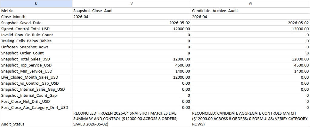
V5 counts invalid or blank cells across the three tables. V6 is the guard for rows added below a table. It counts every filled cell in columns A to G, I to L, and N to S, then subtracts the cells inside each table. Anything below the tables, whether in row 10 or row 500, makes it greater than 0 and stops the checks. V7 counts the snapshot rows that still hold formulas.
V8 passes the frozen order count through only when the close stamp is valid. The stamp must be typed values, not formulas, and the close date must be on or after the last day of the close month, which the formula finds with EOMONTH. V9 to V11 read the frozen total and the largest and smallest service lines. V12 reads the live total. V13 compares the snapshot with the control total, and V14 and V15 check that the frozen total row matches its own lines. V16 is the net change since close, ROUND(V12-V9, 2). V17 adds up how far each service line has moved in column S.
At baseline, V18 says:
RECONCILED: FROZEN 2026-04 SNAPSHOT MATCHES LIVE SUMMARY AND CONTROL ($12000.00 ACROSS 8 ORDERS; SAVED 2026-05-02)
Each change below was made on its own in the test. To repeat one, start from a fresh duplicate of the untouched Month_Close tab, make that single change on the copy, and delete the copy afterward:
| Change on a copy of Month_Close | V18 says |
|---|---|
D5 = 1200, the late credit |
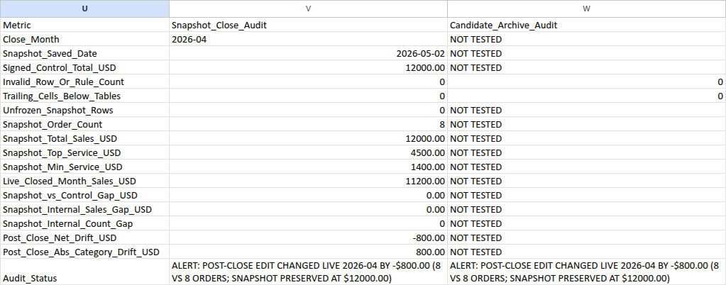
ALERT: POST-CLOSE EDIT CHANGED LIVE 2026-04 BY -$800.00 (8 VS 8 ORDERS; SNAPSHOT PRESERVED AT $12000.00) |
| $100.00 moved from Software to Support | ALERT: POST-CLOSE CATEGORY SHIFT OF $200.00 ACROSS SERVICE LINES (SNAPSHOT PRESERVED AT $12000.00) |
Regular paste of I2:K6 into N2:P6 |
STOP: SNAPSHOT NOT FROZEN (5 ROWS STILL HAVE LIVE FORMULAS) |
Paste values over J2:K6 |
STOP: LIVE SUMMARY FORMULAS OVERWRITTEN WITH STATIC VALUES (RESTORE LIVE FORMULAS) |
V3 = =TODAY() |
STOP: VOLATILE OR FORMULA CLOSE STAMP (ENTER STATIC VALUES IN V2:V4) |
V3 = 2026-04-29 |
STOP: PREMATURE SNAPSHOT DATE (SAVED BEFORE MONTH-END) |
P6 = 12500 |
STOP: SNAPSHOT TOTAL ROW DOES NOT MATCH SUM OF SNAPSHOT LINES |
| A May order typed in row 10, ranges not resized | STOP: TRAILING LEDGER DATA OUTSIDE TABLE RANGE (RESIZE LEDGER) |
The late credit is the case this whole setup exists for. The live total drops to $11,200.00, so V16 shows −800.00, and the snapshot in P6 still reads $12,000.00. A close date of 2026-04-30, the last day of April, reconciles. One day earlier stops.
The $100.00 move shows $200.00 because Software and Support each moved $100.00, and V17 adds both. The net change in V16 stays at 0.00. If an edit changes how many orders each service line has but leaves every line’s dollars the same, V18 reads CATEGORY SHIFT OF $0.00. That doesn’t mean nothing moved. Look at column R. In the test, R3 and R4 each showed 1.
Checking another saved copy. Until you have readings, leave W2:W4 and W7:W11 at NOT TESTED and W5:W6 at 0. To check a copy, type its close month in W2, its saved date in W3, and its control total in W4. Then type the number of its saved rows that still hold a formula in W7, and its four totals in W8:W11. Keep W5 and W6 at 0. Set everything back to NOT TESTED and 0 after each check, so one test doesn’t carry into the next.
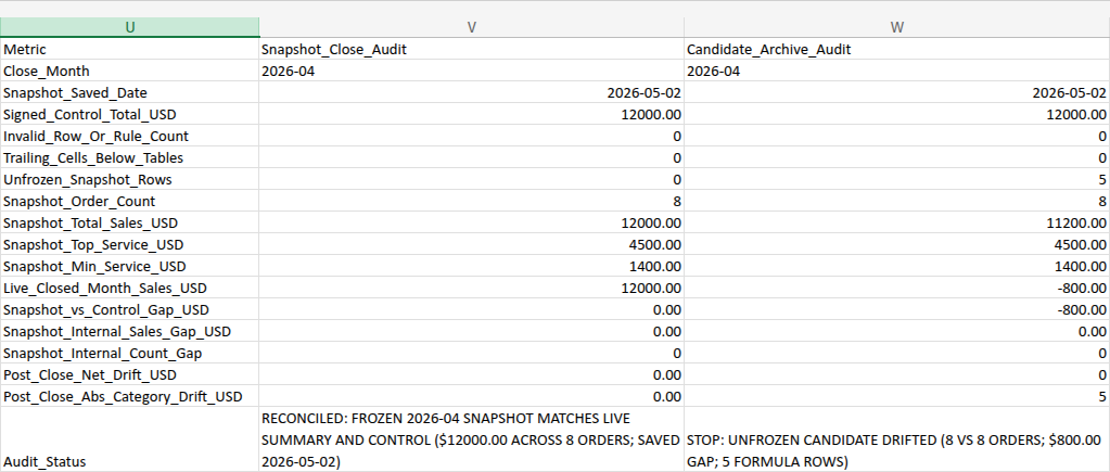
Count W7 by row, not by cell. Look at the five saved summary rows in the other copy, from Hardware to the total row, and count a row once if any of its saved cells holds a formula. Don’t count check columns like Q to S, which are formulas on purpose. A regular paste puts formulas in 10 cells, the count and the dollars of 5 rows, so W7 is 5. If the saved rows are all plain values but the close date is a formula, as with =TODAY(), enter 1 for that one cell. That’s the =TODAY() row in the table below, which reports 1 FORMULA CELL.
W5 and W6 don’t inspect the other copy. They’re guard cells that must stay 0 for column W to run, so check the other copy’s rows and anything below its tables yourself.
| Saved copy being checked | W2, W3, W4, W7, W8, W9, W10, W11 | W18 says |
|---|---|---|
| Frozen correctly | 2026-04, 2026-05-02, 12000, 0, 8, 12000, 4500, 1400 | RECONCILED: CANDIDATE AGGREGATE CONTROLS MATCH ($12000.00 ACROSS 8 ORDERS; 0 FORMULAS; VERIFY CATEGORY ROWS) |
| Regular paste, then the late credit | 2026-04, 2026-05-02, 12000, 5, 8, 11200, 4500, 1400 | STOP: UNFROZEN CANDIDATE DRIFTED (8 VS 8 ORDERS; $800.00 GAP; 5 FORMULA ROWS) |
=TODAY() close date, opened 16 days later |
2026-04, 2026-05-18, 12000, 1, 8, 12000, 4500, 1400 | STOP: VOLATILE CLOSE DATE SHIFTED BY 16 DAYS (1 FORMULA CELL) |
| Frozen on April 25 | 2026-04, 2026-04-25, 12000, 0, 6, 9700, 3500, 1400 | STOP: CANDIDATE SAVED BEFORE MONTH-END (2026-04-25) |
| Stale 6-order export pasted May 2 | 2026-04, 2026-05-02, 12000, 0, 6, 9700, 3500, 1400 | STOP: CANDIDATE ORDER COUNT MISMATCH (6 VS 8; $2300.00 CONTROL GAP) |
In the test, the regular-paste and 6-order readings came from probe copies built in both programs. The 6-order copy had 2 Hardware orders for $3,300.00, 2 Software for $3,500.00, 1 Support for $1,500.00, and 1 Training for $1,400.00. The 16-day reading was typed in to show the arithmetic. The real =TODAY() in the test returned the test date.
When column V stops, column W shows the same message, so fix the workbook before you check any other copy. Even a reconciled W18 ends with VERIFY CATEGORY ROWS, and the last section explains why.
Adding May Without Losing April
You can add May orders to the same ledger. With V2 still set to 2026-04, column G marks them "OTHER MONTH", and the April summary ignores them. In the test, adding a ninth order dated 2026-05-04 left April reconciled at $12,000.00.
Don’t just change V2 to 2026-05. In the test, doing that with the close date still at 2026-05-02 stopped with STOP: PREMATURE SNAPSHOT DATE (SAVED BEFORE MONTH-END). And pasting May’s values into N2:P6 would replace April’s snapshot. Before you reuse the block for May, save April’s frozen values with its close month, close date, and control total somewhere else, such as a values-only copy of the tab or an archive file made as described in Step 2. Automatic drift checks for an archived month are outside this walkthrough.
Before you change the layout. Resizing the ledger or adding a service line rewrites formulas and moves cells, including protected ones. Have the owner lift protection for the change. In Excel for the web, choose Review > Manage Protection and use Pause Protection, or turn Protect sheet off. In Google Sheets, owners can edit restricted ranges, and anyone else needs the protection removed first. Turn protection back on right after. Then check that it still covers the saved values and V2:V4, including any rows the change moved, and check V18: it stays unchanged after a layout-only resize or a next-month row, and it raises an ALERT when an added row changes the closed month.
To add orders to the ledger, type them in columns A to D below the last row, and leave E to G empty in those rows for now. Then update the formula ranges with Find and Replace. Every range ends at a fixed last row, so a resize means replacing the old last row with the new one.
- Select from
E2across to column W, down to the largest of row 18, the ledger’s last row, and the summary’s total row. In the example, that’sE2:W18. - Replace
:$A$9with:$A$10. Do the same for columns B to G, so seven replacements in all. - Copy
E2:G2down to row 10. If the sheet is protected in Excel for the web, extend Unlocked ranges fromA2:D9toA2:D10(in Google Sheets, keep the new ledger rows outside the protected ranges) before turning protection back on.
The selection has to reach every summary row. In the test, a workbook with 20 service lines had its total row in row 22. Resizing with only E2:W18 missed the last service lines, and an April order worth $900.00 never reached the summary while the checks still read reconciled. With E2:W22, the checks caught it: ALERT: POST-CLOSE EDIT CHANGED LIVE 2026-04 BY +$900.00 (9 VS 8 ORDERS; SNAPSHOT PRESERVED AT $12000.00).
Keep Find and Replace inside your selection and make it search the formulas:
- Google Sheets: choose Edit > Find and replace, set Search to Specific range, and check Also search within formulas. It’s unchecked by default. Leave Match entire cell contents unchecked.
- Excel for the web: choose Home > Find & Select > Replace, set Within to Selection under the search options, and leave Match entire cell contents unchecked. The tested dialog had no option for searching formulas, and Replace All changed the formula text directly.
To add a service line, move the total rows in the summary and the snapshot together, without touching the ledger or the check block. Select I6:S6 and insert cells, shifting down. In Google Sheets, that’s Insert > Cells > Insert cells and shift down. In Excel for the web, it’s Home > Insert > Insert Cells & Shift Down, under Show More Options if you don’t see it. Both totals move to row 7, and the formulas that point at the total rows update themselves. Type the new line in I6, and type its frozen values in N6:P6, such as 0 and 0 for a line with no sales in the closed month. Then select from E2 across to column W, down to the largest of row 18, the ledger’s last row, and the new total row. In the example, that’s E2:W18. Replace :$I$5 with :$I$6, and do the same for columns J to L and N to S, and copy J2:L2 and Q2:S2 down to row 6. In the test, adding an Installation line at $0.00 reconciled in both programs.
Never insert or delete whole worksheet rows. That moves or cuts the blocks beside the one you’re changing.
What These Checks Can’t Prove
Column W compares totals, not each line. It checks the order count, the total, and the largest and smallest service lines. A copy with Software at $3,400.00 and Support at $2,700.00, instead of $3,500.00 and $2,600.00, has the same count, total, largest, and smallest line. In the test, W18 still reconciled. A copy with two service-line names swapped, or with order counts moved between two lines, can pass the same way. Compare each line of the other copy with N2:P5. On Month_Close itself, columns R and S do check every line, which is why the same $100.00 move raised an alert there.
Offsetting edits inside one service line don’t show. If one Hardware order drops by $200.00 and another rises by $200.00, Hardware still shows 3 orders and $4,500.00, and the checks stay reconciled. If you need an order-by-order record of the closed month, save a values-only copy of the closed month’s ledger rows along with the summary.
ISFORMULA confirms a formula is there, not that it’s right. That’s the =4500 case from Step 1.
The control total is only as good as the tie-out. The sheet can confirm that the snapshot matches V4. It can’t confirm that V4 matches your accounting or point-of-sale system. A person has to check that at close.
Frequently Asked Questions
Should I keep the snapshot next to the live summary, on its own tab, or in a separate file?
Next to the live summary is the simplest, because the freeze checks and drift checks work as soon as you paste. A separate tab per month keeps the main sheet tidy, but it needs its own typed close stamp and formulas that point back at the live sheet. A separate archive file keeps closed months away from day-to-day editors and keeps the main file small. If you use one, freeze a values-only copy inside the source workbook before you copy it out.
Isn’t version history enough?
It’s a good backup, but it can’t do the job alone. In Google Sheets, only editors can see it, and you can name up to 15 versions per spreadsheet. In Excel, it needs OneDrive or SharePoint, and personal accounts keep the last 25 versions. In both, restoring an earlier version changes the live file, and no formula can compare the current numbers with an old version. A frozen snapshot in the workbook can.
What if an invoice changes after the month closes?
Leave the snapshot as it is. It records what you reported at close. V16 and V18 show the exact change, such as the −$800.00 credit in the example, so you can decide what to do with it. Either record the change as an adjustment in the next month, or save a corrected snapshot for April with a new date and a note that explains it. Don’t overwrite the old snapshot without a record.
What to Do Next
Make the freeze part of your close: confirm the month loaded, type the close stamp and control total, check the live totals, paste values into the snapshot, protect it, and read V18 before you share the numbers. Closed months that stay put are what make month-over-month reports like a monthly KPI scorecard or a budget vs. actual variance worth comparing. If your service-line or customer names come in spelled several ways, map them to stable IDs before the summary counts them.
Formula Reference
Each label before = names the destination cell; paste only the formula. Fill E2:G2 down to row 9, J2:L2 down to row 5, and Q2:S2 down to row 6. Paste J6, K6, L6, and the column V and W formulas one cell at a time.
Headings: A1:G1 are order_id, order_date, service_line, net_sales_usd, Row_Check, Order_Month, and Close_Scope_Status. I1:L1 are service_line, live_order_count, live_net_sales_usd, and Live_Formula_Check. N1:S1 are snapshot_service_line, snapshot_order_count, snapshot_net_sales_usd, Snapshot_Freeze_Check, Abs_Row_Count_Drift, and Abs_Row_Sales_Drift_USD. U1:W1 are Metric, Snapshot_Close_Audit, and Candidate_Archive_Audit, with the metric labels from the check-block table in U2:U18.
Typed inputs: I2:I5 = Hardware, Software, Support, and Training, I6 = Summary_Total, N2:P6 = the pasted values, V2 = ‘2026-04, V3 = 2026-05-02, V4 = 12000, W2:W4 and W7:W11 = NOT TESTED, and W5:W6 = 0.
Ledger helpers:
E2: =IF(OR(COUNTA(A2:D2)<4, NOT(ISTEXT(A2)), NOT(ISNUMBER(B2)), NOT(ISTEXT(C2)), NOT(ISNUMBER(D2))), "CHECK ROW", IF(OR(TRIM(SUBSTITUTE(A2, CHAR(160), " "))="", TRIM(SUBSTITUTE(C2, CHAR(160), " "))="", NOT(EXACT(A2, TRIM(SUBSTITUTE(A2, CHAR(160), " ")))), NOT(EXACT(A2, UPPER(A2))), NOT(EXACT(C2, TRIM(SUBSTITUTE(C2, CHAR(160), " ")))), NOT(ISERROR(FIND(" ", A2))), NOT(ISERROR(FIND(CHAR(10), A2&C2))), NOT(ISERROR(FIND(CHAR(13), A2&C2))), NOT(ISERROR(FIND("*", A2&C2))), NOT(ISERROR(FIND("?", A2&C2))), NOT(ISERROR(FIND("~", A2&C2))), NOT(ISERROR(FIND("=", A2&C2))), NOT(ISERROR(FIND("<", A2&C2))), NOT(ISERROR(FIND(">", A2&C2))), COUNTIF($A$2:$A$9, "*")<ROWS($A$2:$A$9)), "CHECK ROW", IF(OR(INT(B2)<>B2, B2<DATE(2000,1,1), B2>DATE(2100,1,1), D2<0, ROUND(D2, 2)<>D2, SUMPRODUCT(--(UPPER($A$2:$A$9)=UPPER(A2)))>1), "CHECK ROW", "OK")))
F2: =IF(NOT(EXACT(E2, "OK")), "", TEXT(B2, "yyyy-mm"))
G2: =IF(OR(NOT(EXACT(E2, "OK")), COUNTIF($E$2:$E$9, "OK")<ROWS($A$2:$A$9), ISFORMULA($V$2), NOT(ISTEXT($V$2))), "CHECK INPUTS", IF(OR(LEN($V$2)<>7, NOT(EXACT($V$2, TRIM(SUBSTITUTE($V$2, CHAR(160), " "))))), "CHECK INPUTS", IF(NOT(EXACT(F2, $V$2)), "OTHER MONTH", IF(COUNTIF($I$2:$I$5, "*")<ROWS($I$2:$I$5), "CHECK INPUTS", IF(SUMPRODUCT(--(UPPER($I$2:$I$5)=UPPER(C2)))=0, "UNLISTED SERVICE LINE", "IN CLOSED MONTH")))))
Live summary:
J2: =IF(OR(COUNTIF($E$2:$E$9, "OK")<ROWS($A$2:$A$9), COUNTIF($G$2:$G$9, "CHECK INPUTS")>0, COUNTIF($I$2:$I$5, "*")<ROWS($I$2:$I$5), NOT(ISTEXT($I2))), "CHECK INPUTS", IF(OR(TRIM(SUBSTITUTE($I2, CHAR(160), " "))="", NOT(EXACT($I2, TRIM(SUBSTITUTE($I2, CHAR(160), " ")))), NOT(ISERROR(FIND(CHAR(10), $I2))), NOT(ISERROR(FIND(CHAR(13), $I2))), NOT(ISERROR(FIND("*", $I2))), NOT(ISERROR(FIND("?", $I2))), NOT(ISERROR(FIND("~", $I2))), NOT(ISERROR(FIND("=", $I2))), NOT(ISERROR(FIND("<", $I2))), NOT(ISERROR(FIND(">", $I2))), SUMPRODUCT(--(UPPER($I$2:$I$5)=UPPER($I2)))>1), "CHECK INPUTS", COUNTIFS($F$2:$F$9, $V$2, $C$2:$C$9, $I2)))
K2: =IF(NOT(ISNUMBER(J2)), "CHECK INPUTS", ROUND(SUMIFS($D$2:$D$9, $F$2:$F$9, $V$2, $C$2:$C$9, $I2), 2))
L2: =IF(OR(NOT(ISFORMULA(J2)), NOT(ISFORMULA(K2))), "BROKEN: STATIC OVERWRITE", IF(OR(NOT(ISNUMBER(J2)), NOT(ISNUMBER(K2))), "CHECK INPUTS", "LIVE FORMULA"))
J6: =IF(NOT(ISTEXT($I$6)), "CHECK INPUTS", IF(OR(NOT(EXACT($I$6, "Summary_Total")), COUNT($J$2:$J$5)<ROWS($I$2:$I$5)), "CHECK INPUTS", SUM($J$2:$J$5)))
K6: =IF(OR(NOT(ISNUMBER($J$6)), COUNT($K$2:$K$5)<ROWS($I$2:$I$5)), "CHECK INPUTS", ROUND(SUM($K$2:$K$5), 2))
L6: =IF(OR(NOT(ISFORMULA(J6)), NOT(ISFORMULA(K6))), "BROKEN: STATIC OVERWRITE", IF(OR(NOT(ISNUMBER(J6)), NOT(ISNUMBER(K6))), "CHECK INPUTS", "LIVE FORMULA"))
Snapshot checks:
Q2: =IF(OR(ISFORMULA(N2), ISFORMULA(O2), ISFORMULA(P2)), "UNFROZEN FORMULA", IF(OR(COUNTA(N2:P2)<3, NOT(ISTEXT(N2)), NOT(ISNUMBER(O2)), NOT(ISNUMBER(P2))), "CHECK SNAPSHOT", IF(OR(TRIM(SUBSTITUTE(N2, CHAR(160), " "))="", NOT(EXACT(N2, TRIM(SUBSTITUTE(N2, CHAR(160), " ")))), NOT(ISERROR(FIND(CHAR(10), N2))), NOT(ISERROR(FIND(CHAR(13), N2))), NOT(ISERROR(FIND("*", N2))), NOT(ISERROR(FIND("?", N2))), NOT(ISERROR(FIND("~", N2))), NOT(ISERROR(FIND("=", N2))), NOT(ISERROR(FIND("<", N2))), NOT(ISERROR(FIND(">", N2))), INT(O2)<>O2, O2<0, P2<0, ROUND(P2, 2)<>P2), "CHECK SNAPSHOT", "FROZEN VALUE")))
R2: =IF(OR(NOT(EXACT(Q2, "FROZEN VALUE")), NOT(ISNUMBER(J2)), NOT(ISTEXT(I2))), "CHECK INPUTS", IF(NOT(EXACT(N2, I2)), "LABEL MISMATCH", ABS(J2-O2)))
S2: =IF(OR(NOT(ISNUMBER(R2)), NOT(ISNUMBER(K2))), "CHECK INPUTS", ROUND(ABS(K2-P2), 2))
Close checks:
V5: =COUNTIF($E$2:$E$9, "<>OK")+COUNTBLANK($A$2:$A$9)+COUNTBLANK($B$2:$B$9)+COUNTBLANK($C$2:$C$9)+COUNTBLANK($D$2:$D$9)+COUNTIF($G$2:$G$9, "UNLISTED SERVICE LINE")+COUNTIF($G$2:$G$9, "CHECK INPUTS")+COUNTBLANK($I$2:$I$5)+IF(ISTEXT($I$6), IF(EXACT($I$6, "Summary_Total"), 0, 1), 1)+COUNTIF($L$2:$L$5, "<>LIVE FORMULA")+IF(EXACT($L$6, "LIVE FORMULA"), 0, 1)+COUNTBLANK($N$2:$N$5)+COUNTBLANK($O$2:$O$5)+COUNTBLANK($P$2:$P$5)+IF(COUNTA($N$6:$P$6)<3, 1, 0)+COUNTIF($Q$2:$Q$5, "<>FROZEN VALUE")+IF(EXACT($Q$6, "FROZEN VALUE"), 0, 1)+COUNTIF($R$2:$R$5, "LABEL MISMATCH")+IF(EXACT($R$6, "LABEL MISMATCH"), 1, 0)
V6: =(COUNTA($A:$G)-COUNTA($A$1:$G$9))+(COUNTA($I:$L)-COUNTA($I$1:$L$6))+(COUNTA($N:$S)-COUNTA($N$1:$S$6))
V7: =COUNTIF($Q$2:$Q$5, "UNFROZEN FORMULA")+IF(EXACT($Q$6, "UNFROZEN FORMULA"), 1, 0)
V8: =IF(OR(ISFORMULA($V$2), ISFORMULA($V$3), ISFORMULA($V$4), NOT(ISTEXT($V$2)), NOT(ISNUMBER($V$3)), NOT(ISNUMBER($V$4))), "CHECK INPUTS", IF(OR(LEN($V$2)<>7, NOT(EXACT($V$2, TRIM(SUBSTITUTE($V$2, CHAR(160), " ")))), NOT(EXACT(MID($V$2, 5, 1), "-")), NOT(ISNUMBER(FIND(MID($V$2, 1, 1), "0123456789"))), NOT(ISNUMBER(FIND(MID($V$2, 2, 1), "0123456789"))), NOT(ISNUMBER(FIND(MID($V$2, 3, 1), "0123456789"))), NOT(ISNUMBER(FIND(MID($V$2, 4, 1), "0123456789"))), NOT(ISNUMBER(FIND(MID($V$2, 6, 1), "0123456789"))), NOT(ISNUMBER(FIND(MID($V$2, 7, 1), "0123456789")))), "CHECK INPUTS", IF(OR(VALUE(LEFT($V$2, 4))<2000, VALUE(LEFT($V$2, 4))>2100, VALUE(RIGHT($V$2, 2))<1, VALUE(RIGHT($V$2, 2))>12, INT($V$3)<>$V$3, $V$3<DATE(2000,1,1), $V$3>DATE(2100,1,1), $V$4<0, ROUND($V$4, 2)<>$V$4, V5>0, V6>0, V7>0, NOT(ISNUMBER($J$6)), NOT(ISNUMBER($K$6)), COUNT($R$2:$R$5)<ROWS($N$2:$N$5), NOT(ISNUMBER($R$6)), COUNT($S$2:$S$5)<ROWS($N$2:$N$5), NOT(ISNUMBER($S$6))), "CHECK INPUTS", IF($V$3<EOMONTH(DATE(VALUE(LEFT($V$2, 4)), VALUE(RIGHT($V$2, 2)), 1), 0), "CHECK INPUTS", $O$6))))
V9: =IF(NOT(ISNUMBER(V8)), "CHECK INPUTS", ROUND($P$6, 2))
V10: =IF(NOT(ISNUMBER(V8)), "CHECK INPUTS", ROUND(MAX($P$2:$P$5), 2))
V11: =IF(NOT(ISNUMBER(V8)), "CHECK INPUTS", ROUND(MIN($P$2:$P$5), 2))
V12: =IF(NOT(ISNUMBER(V8)), "CHECK INPUTS", ROUND($K$6, 2))
V13: =IF(NOT(ISNUMBER(V8)), "CHECK INPUTS", ROUND(V9-$V$4, 2))
V14: =IF(NOT(ISNUMBER(V8)), "CHECK INPUTS", ROUND($P$6-SUM($P$2:$P$5), 2))
V15: =IF(NOT(ISNUMBER(V8)), "CHECK INPUTS", $O$6-SUM($O$2:$O$5))
V16: =IF(NOT(ISNUMBER(V8)), "CHECK INPUTS", ROUND(V12-V9, 2))
V17: =IF(NOT(ISNUMBER(V8)), "CHECK INPUTS", ROUND(SUM($S$2:$S$5), 2))
V18: =IF(OR(COUNTIF($E$2:$E$9, "<>OK")>0, COUNTBLANK($A$2:$A$9)+COUNTBLANK($B$2:$B$9)+COUNTBLANK($C$2:$C$9)+COUNTBLANK($D$2:$D$9)>0), "STOP: INVALID OR BLANK LEDGER ROWS", IF(OR(ISFORMULA($V$2), ISFORMULA($V$3), ISFORMULA($V$4)), "STOP: VOLATILE OR FORMULA CLOSE STAMP (ENTER STATIC VALUES IN V2:V4)", IF(IF(AND(ISTEXT($V$2), ISNUMBER($V$3), ISNUMBER($V$4)), IF(AND(LEN($V$2)=7, EXACT($V$2, TRIM(SUBSTITUTE($V$2, CHAR(160), " "))), EXACT(MID($V$2, 5, 1), "-"), ISNUMBER(FIND(MID($V$2, 1, 1), "0123456789")), ISNUMBER(FIND(MID($V$2, 2, 1), "0123456789")), ISNUMBER(FIND(MID($V$2, 3, 1), "0123456789")), ISNUMBER(FIND(MID($V$2, 4, 1), "0123456789")), ISNUMBER(FIND(MID($V$2, 6, 1), "0123456789")), ISNUMBER(FIND(MID($V$2, 7, 1), "0123456789"))), OR(VALUE(LEFT($V$2, 4))<2000, VALUE(LEFT($V$2, 4))>2100, VALUE(RIGHT($V$2, 2))<1, VALUE(RIGHT($V$2, 2))>12, INT($V$3)<>$V$3, $V$3<DATE(2000,1,1), $V$3>DATE(2100,1,1), $V$4<0, ROUND($V$4, 2)<>$V$4), TRUE), TRUE), "STOP: INVALID CLOSE STAMP INPUTS IN V2:V4", IF($V$3<EOMONTH(DATE(VALUE(LEFT($V$2, 4)), VALUE(RIGHT($V$2, 2)), 1), 0), "STOP: PREMATURE SNAPSHOT DATE (SAVED BEFORE MONTH-END)", IF(COUNTA($A:$G)-COUNTA($A$1:$G$9)>0, "STOP: TRAILING LEDGER DATA OUTSIDE TABLE RANGE (RESIZE LEDGER)", IF(COUNTA($I:$L)-COUNTA($I$1:$L$6)>0, "STOP: TRAILING LIVE SUMMARY ROWS (RESIZE SUMMARY)", IF(V6>0, "STOP: TRAILING SNAPSHOT ROWS (RESIZE SNAPSHOT)", IF(OR(COUNTIF($L$2:$L$5, "BROKEN: STATIC OVERWRITE")>0, EXACT($L$6, "BROKEN: STATIC OVERWRITE")), "STOP: LIVE SUMMARY FORMULAS OVERWRITTEN WITH STATIC VALUES (RESTORE LIVE FORMULAS)", IF(COUNTIF($G$2:$G$9, "UNLISTED SERVICE LINE")>0, "STOP: LIVE SUMMARY OMITS UNLISTED SERVICE LINE IN CLOSED MONTH", IF(OR(COUNTIF($L$2:$L$5, "<>LIVE FORMULA")>0, NOT(EXACT($L$6, "LIVE FORMULA")), IF(ISTEXT($I$6), NOT(EXACT($I$6, "Summary_Total")), TRUE)), "STOP: INVALID LIVE SUMMARY CATEGORY LABELS", IF(V7>0, "STOP: SNAPSHOT NOT FROZEN (" & V7 & IF(V7=1, " ROW STILL HAS LIVE FORMULAS)", " ROWS STILL HAVE LIVE FORMULAS)"), IF(OR(COUNTIF($Q$2:$Q$5, "<>FROZEN VALUE")>0, NOT(EXACT($Q$6, "FROZEN VALUE"))), "STOP: INVALID OR BLANK CELLS IN FROZEN SNAPSHOT", IF(OR(COUNTIF($R$2:$R$5, "LABEL MISMATCH")>0, EXACT($R$6, "LABEL MISMATCH")), "STOP: SNAPSHOT CATEGORY LABELS DO NOT MATCH LIVE SUMMARY", IF(NOT(ISNUMBER(V8)), "STOP: CHECK SNAPSHOT OR SUMMARY STRUCTURE", IF(OR(V14<>0, V15<>0), "STOP: SNAPSHOT TOTAL ROW DOES NOT MATCH SUM OF SNAPSHOT LINES", IF(V13<>0, "STOP: SNAPSHOT DIFFERS FROM SIGNED CONTROL TOTAL BY $" & TEXT(ABS(V13), "0.00"), IF(OR(V16<>0, $J$6<>V8), "ALERT: POST-CLOSE EDIT CHANGED LIVE " & $V$2 & " BY " & IF(V16>=0, "+$", "-$") & TEXT(ABS(V16), "0.00") & " (" & $J$6 & " VS " & V8 & " ORDERS; SNAPSHOT PRESERVED AT $" & TEXT(V9, "0.00") & ")", IF(OR(V17<>0, SUM($R$2:$R$5)>0), "ALERT: POST-CLOSE CATEGORY SHIFT OF $" & TEXT(V17, "0.00") & " ACROSS SERVICE LINES (SNAPSHOT PRESERVED AT $" & TEXT(V9, "0.00") & ")", "RECONCILED: FROZEN " & $V$2 & " SNAPSHOT MATCHES LIVE SUMMARY AND CONTROL ($" & TEXT(V9, "0.00") & " ACROSS " & V8 & " ORDERS; SAVED " & TEXT($V$3, "yyyy-mm-dd") & ")"))))))))))))))))))
Checks for another saved copy:
W12: =IF(EXACT(W16, "NOT TESTED"), "NOT TESTED", IF(OR(NOT(ISNUMBER(W16)), NOT(ISNUMBER(V9)), NOT(ISNUMBER(W9))), "CHECK INPUTS", ROUND(W9-V9, 2)))
W13: =IF(EXACT(W16, "NOT TESTED"), "NOT TESTED", IF(OR(NOT(ISNUMBER(W16)), NOT(ISNUMBER($V$4)), NOT(ISNUMBER(W9))), "CHECK INPUTS", ROUND(W9-$V$4, 2)))
W14: =IF(EXACT(W16, "NOT TESTED"), "NOT TESTED", IF(OR(NOT(ISNUMBER(W16)), NOT(ISNUMBER(V10)), NOT(ISNUMBER(V11)), NOT(ISNUMBER(W10)), NOT(ISNUMBER(W11))), "CHECK INPUTS", ROUND(ABS(W10-V10)+ABS(W11-V11), 2)))
W15: =IF(EXACT(W16, "NOT TESTED"), "NOT TESTED", IF(OR(NOT(ISNUMBER(W16)), NOT(ISNUMBER(V8)), NOT(ISNUMBER(W8))), "CHECK INPUTS", W8-V8))
W16: =IF(OR(V5>0, V6>0, V7>0, NOT(ISNUMBER(V8)), NOT(ISNUMBER(V13)), NOT(ISNUMBER(V14)), NOT(ISNUMBER(V15)), ISFORMULA(W2), ISFORMULA(W3), ISFORMULA(W4), ISFORMULA(W5), ISFORMULA(W6), ISFORMULA(W7), ISFORMULA(W8), ISFORMULA(W9), ISFORMULA(W10), ISFORMULA(W11), NOT(ISNUMBER(W5)), NOT(ISNUMBER(W6))), "CHECK INPUTS", IF(OR(V13<>0, V14<>0, V15<>0, INT(W5)<>W5, W5<>0, INT(W6)<>W6, W6<>0), "CHECK INPUTS", IF(IF(AND(ISTEXT(W2), ISTEXT(W3), ISTEXT(W4), ISTEXT(W7), ISTEXT(W8), ISTEXT(W9), ISTEXT(W10), ISTEXT(W11)), AND(EXACT(W2, "NOT TESTED"), EXACT(W3, "NOT TESTED"), EXACT(W4, "NOT TESTED"), EXACT(W7, "NOT TESTED"), EXACT(W8, "NOT TESTED"), EXACT(W9, "NOT TESTED"), EXACT(W10, "NOT TESTED"), EXACT(W11, "NOT TESTED")), FALSE), "NOT TESTED", IF(OR(NOT(ISTEXT(W2)), NOT(ISNUMBER(W3)), NOT(ISNUMBER(W4)), NOT(ISNUMBER(W7)), NOT(ISNUMBER(W8)), NOT(ISNUMBER(W9)), NOT(ISNUMBER(W10)), NOT(ISNUMBER(W11))), "CHECK INPUTS", IF(OR(NOT(EXACT(W2, $V$2)), INT(W3)<>W3, W3<DATE(2000,1,1), W3>DATE(2100,1,1), W4<0, ROUND(W4, 2)<>W4, ROUND(W4, 2)<>ROUND($V$4, 2), INT(W7)<>W7, W7<0, INT(W8)<>W8, W8<0, W9<0, ROUND(W9, 2)<>W9, W10<0, ROUND(W10, 2)<>W10, W11<0, ROUND(W11, 2)<>W11, W10<W11, W10>W9, AND(W8=0, W9>0)), "CHECK INPUTS", W3-$V$3)))))
W17: =IF(EXACT(W16, "NOT TESTED"), "NOT TESTED", IF(OR(NOT(ISNUMBER(W16)), NOT(ISNUMBER(W7))), "CHECK INPUTS", W7))
W18: =IF(LEFT(V18, 5)="STOP:", V18, IF(IF(AND(NOT(ISFORMULA(W5)), NOT(ISFORMULA(W6)), ISNUMBER(W5), ISNUMBER(W6)), OR(INT(W5)<>W5, W5<>0, INT(W6)<>W6, W6<>0), TRUE), "STOP: INVALID CANDIDATE GUARD INPUTS", IF(EXACT(W16, "NOT TESTED"), IF(LEFT(V18, 6)="ALERT:", V18, "NOT TESTED: ENTER CANDIDATE ARCHIVE READINGS"), IF(EXACT(W16, "CHECK INPUTS"), "STOP: NON-NUMERIC, MISMATCHED CONTROL, OR INCOMPLETE CANDIDATE INPUTS", IF(W3<EOMONTH(DATE(VALUE(LEFT($V$2, 4)), VALUE(RIGHT($V$2, 2)), 1), 0), "STOP: CANDIDATE SAVED BEFORE MONTH-END (" & TEXT(W3, "yyyy-mm-dd") & ")", IF(W17>0, IF(OR(W12<>0, W15<>0), "STOP: UNFROZEN CANDIDATE DRIFTED (" & W8 & " VS " & V8 & " ORDERS; $" & TEXT(ABS(W12), "0.00") & " GAP; " & W17 & IF(W17=1, " FORMULA ROW)", " FORMULA ROWS)"), IF(W14>0, "STOP: UNFROZEN CANDIDATE SHIFTED SERVICE TOTALS BY $" & TEXT(W14, "0.00") & " (" & W17 & IF(W17=1, " FORMULA ROW)", " FORMULA ROWS)"), IF(W16<>0, "STOP: VOLATILE CLOSE DATE SHIFTED BY " & ABS(W16) & IF(ABS(W16)=1, " DAY (", " DAYS (") & W17 & IF(W17=1, " FORMULA CELL)", " FORMULA CELLS)"), "STOP: CANDIDATE NOT FROZEN (" & W17 & IF(W17=1, " FORMULA ROW REMAINS)", " FORMULA ROWS REMAIN)")))), IF(W16<>0, "STOP: CANDIDATE SAVE DATE DIFFERS BY " & ABS(W16) & IF(ABS(W16)=1, " DAY", " DAYS") & " FROM CLOSE STAMP", IF(W15<>0, "STOP: CANDIDATE ORDER COUNT MISMATCH (" & W8 & " VS " & V8 & "; $" & TEXT(ABS(W13), "0.00") & " CONTROL GAP)", IF(W13<>0, "STOP: CANDIDATE TOTAL DIFFERS FROM SIGNED CONTROL BY $" & TEXT(ABS(W13), "0.00"), IF(W14>0, "STOP: CANDIDATE SERVICE LINE TOTALS SHIFTED ($" & TEXT(W14, "0.00") & " TOP/MIN DRIFT)", "RECONCILED: CANDIDATE AGGREGATE CONTROLS MATCH ($" & TEXT(W9, "0.00") & " ACROSS " & W8 & " ORDERS; 0 FORMULAS; VERIFY CATEGORY ROWS)"))))))))))