
To find how many extra sales a discount must generate, divide the discount per unit by the gross profit each unit still earns after the discount. The answer is the extra volume you need, as a share of what you sell now, to keep the same gross profit dollars.
Take a $100 item that costs $60 to supply, selling 150 units a month. Each unit earns $40, so the month earns $6,000. At 10% off, the price is $90 and each unit earns $30. $10 ÷ $30 = 33.33%, so you need 200 units, 50 more than now. Selling 10% more, 165 units, earns only $4,950.
The products, prices, and volumes below are made up for educational purposes. Here is how each shortcut comes out:
| Plan for the 10% discount | Units sold | Extra units | Profit per unit | Gross profit | vs. $6,000 |
|---|---|---|---|---|---|
| Break-even: $10 ÷ $30 | 200 | 50 | $30 | $6,000 | $0 |
| Trap 1: sell 10% more | 165 | 15 | $30 | $4,950 | −$1,050 |
| Trap 2: match the old $15,000 revenue | 167 | 17 | $30 | $5,010 | −$990 |
| Trap 3: divide by the old margin, $10 ÷ $40 | 188 | 38 | $30 | $5,640 | −$360 |
| Trap 4: right volume, old $40 margin | 200 | 50 | $40 | $8,000 on paper | +$2,000 that isn’t there |
Why a 10% Discount Needs 33% More Units
The discount comes straight out of profit, but the cost of each unit doesn’t change. Here, $10 off takes a quarter of the $40 profit, so you need a third more units to make it back.
The $60 is cost of sales, so this is gross profit, not net profit or cash.
Matching revenue isn’t enough. $15,000 ÷ $90 is 166.67, so 167 units bring in $15,030. But the 17 extra units cost $60 each, $1,020 in all, and gross profit lands at $5,010.
Dividing by the old margin is the near miss. $10 ÷ $40 gives 25%, or 187.5 units, rounded up to 188. That’s still $360 short.
As rates, the rule is discount ÷ (margin − discount): 10% ÷ (40% − 10%) = 33.33%. Margin on the selling price also drops, from 40% to 33.33%. That’s 6.67 percentage points, not 6.67%, as Percentage Change vs Percentage Points explains.
The rule assumes every unit sells at the discounted price, including the 150 you’d have sold anyway, at the same unit cost. Two common cases break that:
- New-buyer codes. If regulars still pay full price, the $6,000 is already safe, and every added sale at $30 adds profit.
- Waiting and stocking up. Regulars who wait for an announced sale move purchases into it. Buyers who stock up pull later purchases forward. Either way, some of the extra units aren’t new demand, and profit over several months can come out lower.
Step 1: Compare Promotions in One Sheet
Create a tab called Discount_Breakeven. Put the headings below in A1:K1 and the four promotions in A2:F5. Enter discount rates as decimals: 0.1, not 10. Columns G to K are formulas, and the table shows their results.
| Row | promo_id (A) | offer_name (B) | list_price_usd (C) | unit_cost_usd (D) | baseline_units (E) | discount_rate (F) | Row_Check (G) | Baseline_Gross_Profit_USD (H) | Discounted_Unit_Profit_USD (I) | Required_BreakEven_Units (J) | Required_Volume_Lift_Pct (K) |
|---|---|---|---|---|---|---|---|---|---|---|---|
| 2 | PROMO-601 | Standard Maintenance Kit (10% Off) | 100 | 60 | 150 | 0.10 | OK | 6000 | 30 | 200 | 0.3333 |
| 3 | PROMO-602 | Standard Maintenance Kit (20% Off) | 100 | 60 | 150 | 0.20 | OK | 6000 | 20 | 300 | 1.0000 |
| 4 | PROMO-603 | Commercial Filter Pack (10% Off) | 200 | 150 | 60 | 0.10 | OK | 3000 | 30 | 100 | 0.6667 |
| 5 | PROMO-604 | Calibration Service Plan (15% Off) | 80 | 32 | 90 | 0.15 | OK | 4320 | 36 | 120 | 0.3333 |

Enter these five formulas in G2:K2, then copy G2:K2 down to row 5. G2 checks the row:
=IF(OR(COUNTA(A2:F2)<6, NOT(ISTEXT(A2)), NOT(ISTEXT(B2)), TRIM(SUBSTITUTE(A2, CHAR(160), " "))="", TRIM(SUBSTITUTE(B2, CHAR(160), " "))="", NOT(EXACT(A2, TRIM(SUBSTITUTE(A2, CHAR(160), " ")))), NOT(EXACT(B2, TRIM(SUBSTITUTE(B2, CHAR(160), " ")))), LEN(A2)<>9, NOT(EXACT(LEFT(A2, 6), "PROMO-")), NOT(ISNUMBER(FIND(MID(A2, 7, 1), "0123456789"))), NOT(ISNUMBER(FIND(MID(A2, 8, 1), "0123456789"))), NOT(ISNUMBER(FIND(MID(A2, 9, 1), "0123456789"))), NOT(ISNUMBER(C2)), NOT(ISNUMBER(D2)), NOT(ISNUMBER(E2)), NOT(ISNUMBER(F2))), "CHECK INPUTS", IF(OR(C2<=0, ROUND(C2, 2)<>C2, D2<0, ROUND(D2, 2)<>D2, D2>=C2, E2<=0, INT(E2)<>E2, F2<=0, F2>=1, ROUND(C2*(1-F2), 2)>=C2, ROUND(ROUND(C2*(1-F2), 2)-D2, 2)<=0, SUMPRODUCT(--(UPPER($A$2:$A$5)=UPPER(A2)))>1), "CHECK INPUTS", "OK"))
G2 returns CHECK INPUTS for a blank cell, stray spaces, a bad or repeated ID, fractions of a cent, a discount outside 0 to 1, or a price that no longer covers cost. H2:K2 stop unless all four rows say OK.
H2, baseline gross profit:
=IF(OR(NOT(EXACT(G2, "OK")), COUNTIF($G$2:$G$5, "OK")<4), "CHECK INPUTS", ROUND((C2-D2)*E2, 2))
I2, profit per unit after the discount. The discounted price is rounded to whole cents first:
=IF(OR(NOT(EXACT(G2, "OK")), NOT(ISNUMBER(H2)), COUNT($H$2:$H$5)<4), "CHECK INPUTS", ROUND(ROUND(C2*(1-F2), 2)-D2, 2))
J2, break-even units. It divides whole cents and rounds up, because you can’t sell part of a unit:
=IF(OR(NOT(EXACT(G2, "OK")), NOT(ISNUMBER(I2)), COUNT($I$2:$I$5)<4), "CHECK INPUTS", IF(ROUND(I2*100, 0)<=0, "CHECK INPUTS", ROUNDUP(ROUND(H2*100, 0)/ROUND(I2*100, 0), 0)))
K2, the required lift:
=IF(OR(NOT(EXACT(G2, "OK")), NOT(ISNUMBER(J2)), COUNT($J$2:$J$5)<4), "CHECK INPUTS", IF(E2<=0, "CHECK INPUTS", ROUND((J2-E2)/E2, 4)))
At 20% off, unit profit falls to $20, half of $40, and the lift triples, from 33.33% to 100%. At 40% off, each unit earns $0, so no volume makes up the $6,000, and G2 says CHECK INPUTS. The filter pack has a thinner 25% margin, so the same 10% needs 66.67%. The service plan has a 60% margin, so 15% off needs the same 33.33% as the kit at 10%.
So is 10% a safe discount? I wouldn’t pretend to generalize. You’d have to look at that item’s price and cost first.
Set E2 to 100 and J2 shows 134, because 133.33 rounds up. Those 134 units earn $4,020, $20 more than the old $4,000. Set E2 back to 150.
Step 2: Check a Claimed Break-Even Number
I’ve seen numbers that should agree fall out of sync plenty of times. Promotion plans are an easy place for it. This block checks a claimed minimum break-even calculation against the table.
Put Check_Item, Promo_Benchmark, and Candidate_Promo_Audit in M1:O1, and the labels below in M2:M14. Variable_Unit_Cost_USD is the same unit cost of sales as column D. Set N2 to PROMO-601 and O2 to NOT TESTED, and leave O3:O12 blank.
| Row | Label (M) | N shows |
|---|---|---|
| 2 | Target_Promo_ID | PROMO-601 (typed) |
| 3 | List_Price_USD | 100 |
| 4 | Variable_Unit_Cost_USD | 60 |
| 5 | Discount_Rate | 0.1 |
| 6 | Baseline_Units | 150 |
| 7 | Baseline_Gross_Profit_USD | 6000 |
| 8 | Discounted_Unit_Profit_USD | 30 |
| 9 | Required_Total_Units | 200 |
| 10 | Required_Extra_Units | 50 |
| 11 | Required_Volume_Lift_Pct | 0.3333 |
| 12 | Realized_Promo_Gross_Profit_USD | 6000 |
| 13 | Gross_Profit_Variance_USD | 0 |
| 14 | Reconciliation_Status | RECONCILED: +33.33% LIFT … |
N3 starts the benchmark for the promotion in N2:
=IF(OR(NOT(ISTEXT(N2)), COUNTIF($G$2:$G$5, "OK")<4, COUNT($H$2:$H$5)<4, COUNT($I$2:$I$5)<4, COUNT($J$2:$J$5)<4, COUNT($K$2:$K$5)<4), "CHECK INPUTS", IF(SUMPRODUCT(--EXACT($A$2:$A$5, N2))<>1, "CHECK INPUTS", INDEX($C$2:$C$5, MATCH(N2, $A$2:$A$5, 0))))
Then enter N4 to N13:
| Cell | Formula |
|---|---|
| N4 | =IF(NOT(ISNUMBER(N3)), "CHECK INPUTS", INDEX($D$2:$D$5, MATCH(N2, $A$2:$A$5, 0))) |
| N5 | =IF(NOT(ISNUMBER(N3)), "CHECK INPUTS", INDEX($F$2:$F$5, MATCH(N2, $A$2:$A$5, 0))) |
| N6 | =IF(NOT(ISNUMBER(N3)), "CHECK INPUTS", INDEX($E$2:$E$5, MATCH(N2, $A$2:$A$5, 0))) |
| N7 | =IF(NOT(ISNUMBER(N3)), "CHECK INPUTS", INDEX($H$2:$H$5, MATCH(N2, $A$2:$A$5, 0))) |
| N8 | =IF(NOT(ISNUMBER(N3)), "CHECK INPUTS", INDEX($I$2:$I$5, MATCH(N2, $A$2:$A$5, 0))) |
| N9 | =IF(NOT(ISNUMBER(N3)), "CHECK INPUTS", INDEX($J$2:$J$5, MATCH(N2, $A$2:$A$5, 0))) |
| N10 | =IF(NOT(ISNUMBER(N3)), "CHECK INPUTS", N9-N6) |
| N11 | =IF(NOT(ISNUMBER(N3)), "CHECK INPUTS", INDEX($K$2:$K$5, MATCH(N2, $A$2:$A$5, 0))) |
| N12 | =IF(NOT(ISNUMBER(N3)), "CHECK INPUTS", ROUND(N9*N8, 2)) |
| N13 | =IF(NOT(ISNUMBER(N3)), "CHECK INPUTS", ROUND(N12-N7, 2)) |
N14 rechecks the math and writes the status:
=IF(OR(NOT(ISNUMBER(N3)), NOT(ISNUMBER(N4)), NOT(ISNUMBER(N5)), NOT(ISNUMBER(N6)), NOT(ISNUMBER(N7)), NOT(ISNUMBER(N8)), NOT(ISNUMBER(N9)), NOT(ISNUMBER(N10)), NOT(ISNUMBER(N11)), NOT(ISNUMBER(N12)), NOT(ISNUMBER(N13))), "CHECK INPUTS", IF(OR(ROUND(N7-ROUND((N3-N4)*N6, 2), 2)<>0, ROUND(N8-ROUND(ROUND(N3*(1-N5), 2)-N4, 2), 2)<>0, N10<>N9-N6, ROUND(N11-ROUND((N9-N6)/N6, 4), 4)<>0, ROUND(N12-ROUND(N9*N8, 2), 2)<>0, ROUND(N13-ROUND(N12-N7, 2), 2)<>0, ROUND(N13, 2)<0, ROUND(N13-N8, 2)>=0, N9<=N6, N8<=0), "CHECK INPUTS", "RECONCILED: +" & TEXT(N11, "0.00%") & " LIFT (" & N9 & " TOTAL / +" & N10 & " EXTRA UNITS AT $" & TEXT(N8, "0.00") & " MARGIN = $" & TEXT(N12, "0.00") & " PROFIT)"))
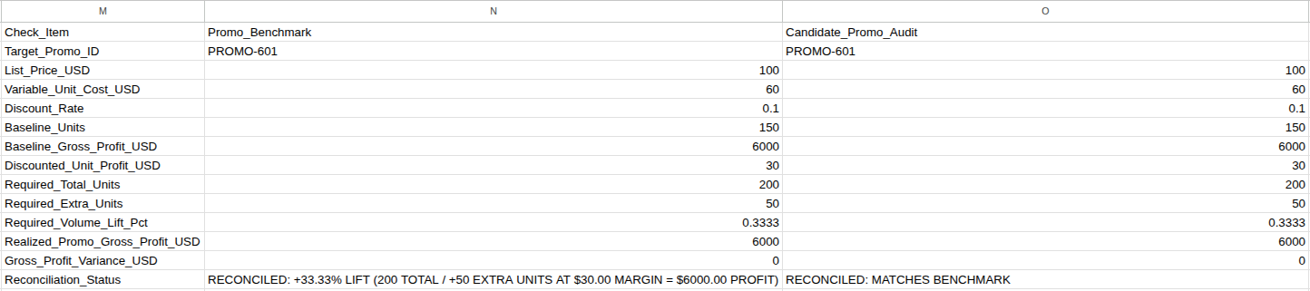
N14 should read RECONCILED: +33.33% LIFT (200 TOTAL / +50 EXTRA UNITS AT $30.00 MARGIN = $6000.00 PROFIT). N13 can land above zero because of rounding up. N14 accepts that as long as it’s less than one unit’s profit, like the $20 above.
Column O checks a break-even claim someone hands you. Copy O13 and O14 from the formula reference at the end. With O2 still NOT TESTED, O14 says NOT TESTED: ENTER CANDIDATE KPI VALUES.
Now try each claim below. Type only into O2:O12, and replace all eleven values each time. O13 and O14 stay formulas; the table shows what they should return. Every test uses O3 = 100, O4 = 60, O6 = 150, and O7 = 6000. O5 is 0.1, except for the PROMO-602 test, which uses 0.2.
| Test | O2 | O8 | O9 | O10 | O11 | O12 | O13 shows | O14 shows (shortened) |
|---|---|---|---|---|---|---|---|---|
| Trap 1 | PROMO-601 | 30 | 165 | 15 | 0.1 | 4950 | −1050 | STOP: 1-FOR-1 PERCENTAGE SWAP TRAP |
| Trap 2 | PROMO-601 | 30 | 167 | 17 | 0.1133 | 5010 | −990 | STOP: REVENUE BREAK-EVEN TRAP |
| Trap 3 | PROMO-601 | 30 | 188 | 38 | 0.2533 | 5640 | −360 | STOP: BREAK-EVEN VOLUME MISMATCH |
| Trap 4 | PROMO-601 | 40 | 200 | 50 | 0.3333 | 8000 | 2000 | STOP: DISCOUNTED UNIT MARGIN MISMATCH |
| Correct | PROMO-601 | 30 | 200 | 50 | 0.3333 | 6000 | 0 | RECONCILED: MATCHES BENCHMARK |
| 20% off | PROMO-602 | 20 | 300 | 150 | 1 | 6000 | 0 | RECONCILED: MATCHES BENCHMARK |
| Overshoot | PROMO-601 | 30 | 210 | 60 | 0.4 | 6300 | 300 | STOP: BREAK-EVEN VOLUME MISMATCH |
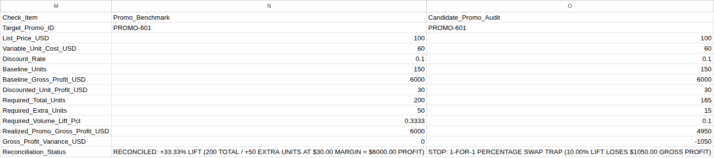
O14 checks inputs, margin, and Traps 1 and 2 before comparing units, extra units, and lift with columns J and K. The overshoot earns $300 more than the old profit. It stops because 210 isn’t the minimum, not because it loses money.
The Trap 1 message shows the lift after rounding to whole units. On PROMO-604, 90 units plus 15% is 103.5, so a claim of 104 units reads 15.56%.
O11 accepts any lift of zero or more, so very deep discounts work: 39% off this item needs a lift of 3,900%. A lift can also round to 0.00% and still need a few extra units, so read O10 as well.
O2 can name another promotion, as in the PROMO-602 test. But column O stops whenever N14 says CHECK INPUTS, so N2 must hold a valid ID. Both match IDs exactly, case included, so promo-602 returns CHECK INPUTS.
To see an input mistake, start from the Correct row and type 10 instead of 0.1 in O5. Only column O returns CHECK INPUTS, and N14 stays reconciled. Change O5 back to 0.1.
These formulas work in Google Sheets and Excel for the web with US English settings. TEXT formats like “0.00%” may need changing in other locales.
Adapting the Sheet to More Promotions
For eight promotions, in this order:
- Enter the new promotions in A6:F9. Don’t insert whole rows, which would shift M:O.
- Select G2:O14 and use Find and Replace, searching inside formulas. Replace
$5with$9(75 places), then<4with<8(21 places). - Only then copy G2:K2 down to row 9, and check that every row says
OK.
For 20 promotions, use $21 and <20, and copy down to row 21. If you copy first, rows below 14 keep checking only rows 2 to 5. For fewer than four, use the smaller numbers, clear the unused cells in A:K only, and keep N2 and O2 valid.
Don’t replace a bare 4 or 5. That would break N4, O5, PROMO-604, and the rounding to four decimals.
Checklist Before You Approve a Discount
- Every row in column G says
OK, and N14 is reconciled. - Any break-even number in the plan matches column J.
- Your sales forecast meets or beats that minimum, and you can fulfill it.
- You know who gets the discount, and how many sales are buyers waiting or stocking up.
- Ad spend and other campaign costs are judged separately.
What to Do Next
Discounting several products? Don’t average their margins. Why you should not average margin percentages shows how to weight them. After the promotion runs, compare the plan with what happened using budget vs. actual variance.
Copy-Paste Formula Reference
O13, the profit variance of the claim:
=IF(OR(EXACT(N14, "CHECK INPUTS"), IF(ISTEXT(O2), NOT(OR(O2="", EXACT(O2, "NOT TESTED"), SUMPRODUCT(--EXACT($A$2:$A$5, O2))=1)), NOT(ISBLANK(O2))), IF(ISNUMBER(O3), OR(O3<=0, ROUND(O3, 2)<>O3), NOT(OR(ISBLANK(O3), O3="", EXACT(O3, "NOT TESTED")))), IF(ISNUMBER(O4), OR(O4<0, ROUND(O4, 2)<>O4), NOT(OR(ISBLANK(O4), O4="", EXACT(O4, "NOT TESTED")))), IF(AND(ISNUMBER(O3), ISNUMBER(O4)), O4>=O3, FALSE), IF(ISNUMBER(O5), OR(O5<=0, O5>=1), NOT(OR(ISBLANK(O5), O5="", EXACT(O5, "NOT TESTED")))), IF(ISNUMBER(O6), OR(O6<=0, INT(O6)<>O6), NOT(OR(ISBLANK(O6), O6="", EXACT(O6, "NOT TESTED")))), IF(ISNUMBER(O7), OR(O7<=0, ROUND(O7, 2)<>O7), NOT(OR(ISBLANK(O7), O7="", EXACT(O7, "NOT TESTED")))), IF(ISNUMBER(O8), OR(O8<=0, ROUND(O8, 2)<>O8), NOT(OR(ISBLANK(O8), O8="", EXACT(O8, "NOT TESTED")))), IF(ISNUMBER(O9), OR(O9<=0, INT(O9)<>O9), NOT(OR(ISBLANK(O9), O9="", EXACT(O9, "NOT TESTED")))), IF(ISNUMBER(O10), OR(O10<0, INT(O10)<>O10), NOT(OR(ISBLANK(O10), O10="", EXACT(O10, "NOT TESTED")))), IF(ISNUMBER(O11), O11<0, NOT(OR(ISBLANK(O11), O11="", EXACT(O11, "NOT TESTED")))), IF(ISNUMBER(O12), OR(O12<=0, ROUND(O12, 2)<>O12), NOT(OR(ISBLANK(O12), O12="", EXACT(O12, "NOT TESTED"))))), "CHECK INPUTS", IF(OR(ISBLANK(O2), O2="", EXACT(O2, "NOT TESTED"), NOT(ISNUMBER(O3)), NOT(ISNUMBER(O4)), NOT(ISNUMBER(O5)), NOT(ISNUMBER(O6)), NOT(ISNUMBER(O7)), NOT(ISNUMBER(O8)), NOT(ISNUMBER(O9)), NOT(ISNUMBER(O10)), NOT(ISNUMBER(O11)), NOT(ISNUMBER(O12))), "NOT TESTED", ROUND(O12-INDEX($H$2:$H$5, MATCH(O2, $A$2:$A$5, 0)), 2)))
O14, the claim’s status:
=IF(EXACT(O13, "CHECK INPUTS"), "CHECK INPUTS", IF(EXACT(O13, "NOT TESTED"), "NOT TESTED: ENTER CANDIDATE KPI VALUES", IF(OR(ROUND(O3-INDEX($C$2:$C$5, MATCH(O2, $A$2:$A$5, 0)), 2)<>0, ROUND(O4-INDEX($D$2:$D$5, MATCH(O2, $A$2:$A$5, 0)), 2)<>0, ROUND(O5-INDEX($F$2:$F$5, MATCH(O2, $A$2:$A$5, 0)), 6)<>0, O6<>INDEX($E$2:$E$5, MATCH(O2, $A$2:$A$5, 0)), ROUND(O7-INDEX($H$2:$H$5, MATCH(O2, $A$2:$A$5, 0)), 2)<>0), "STOP: BASELINE INPUT MISMATCH (CHECK PRICE COST DISCOUNT OR BASELINE UNITS)", IF(ROUND(O8-INDEX($I$2:$I$5, MATCH(O2, $A$2:$A$5, 0)), 2)<>0, "STOP: DISCOUNTED UNIT MARGIN MISMATCH (USE $" & TEXT(INDEX($I$2:$I$5, MATCH(O2, $A$2:$A$5, 0)), "0.00") & " POST-DISCOUNT PROFIT NOT $" & TEXT(O8, "0.00") & ")", IF(AND(O9<INDEX($J$2:$J$5, MATCH(O2, $A$2:$A$5, 0)), OR(O9=ROUNDUP(ROUND(O6*(1+O5), 8), 0), O9=ROUND(O6*(1+O5), 0))), "STOP: 1-FOR-1 PERCENTAGE SWAP TRAP (" & TEXT(ROUND((O9-O6)/O6, 4), "0.00%") & " LIFT LOSES $" & TEXT(ROUND(O7-O9*O8, 2), "0.00") & " GROSS PROFIT)", IF(AND(O9<INDEX($J$2:$J$5, MATCH(O2, $A$2:$A$5, 0)), O4>0, ABS(O9*ROUND(O3*(1-O5), 2)-O6*O3)<ROUND(O3*(1-O5), 2)), "STOP: REVENUE BREAK-EVEN TRAP (IGNORES $" & TEXT(O4, "0.00") & " VARIABLE COST ON EXTRA UNITS)", IF(OR(O9<>INDEX($J$2:$J$5, MATCH(O2, $A$2:$A$5, 0)), O10<>(INDEX($J$2:$J$5, MATCH(O2, $A$2:$A$5, 0))-O6), ROUND(O11-INDEX($K$2:$K$5, MATCH(O2, $A$2:$A$5, 0)), 4)<>0), "STOP: BREAK-EVEN VOLUME MISMATCH (EXPECTED " & INDEX($J$2:$J$5, MATCH(O2, $A$2:$A$5, 0)) & " TOTAL / +" & (INDEX($J$2:$J$5, MATCH(O2, $A$2:$A$5, 0))-O6) & " EXTRA / +" & TEXT(INDEX($K$2:$K$5, MATCH(O2, $A$2:$A$5, 0)), "0.00%") & " LIFT)", IF(OR(ROUND(O12-ROUND(O9*O8, 2), 2)<>0, ROUND(O13, 2)<0, ROUND(O13-O8, 2)>=0), "STOP: REALIZED GROSS PROFIT MISMATCH AT BREAK-EVEN VOLUME", "RECONCILED: MATCHES BENCHMARK"))))))))